目录

• 前言
• 数据采集、处理
• • 导入包
  • 正弦波数据生成
  • 数据集分类
• 模型1训练
• • 模型1创建
  • 模型1训练
  • 检查训练指标
• 模型2训练
• 模型导出（TensorFlow Lite）
• 模型部署、功能编写

前言

TinyML是机器学习前沿的一个分支，致力于在超低功耗、资源受限的边缘端（MCU）部署机器学习模型，实现边缘AI，使机器学习真正大众化，使生活真正智能化。简单来说就是在单片机上跑深度学习，很不可思议吧，因为AI在大众的印象里都是需要大算力、高能耗，TinyML为低功耗AI的普及开了个好头。
下面介绍的一个项目是TinyML最简单入门的一个小项目，麻雀虽小，五脏俱全，它包含了基本的TinyML项目所有的必要步骤。它就是用神经网络训练一个正弦波，然后把正弦波部署到esp32上实现呼吸灯效果，听着很蹩脚，也没什么实用性，因为呼吸灯正常十几行代码就搞定了，但这主要是为了入门TinyML嘛，最终我们自己训练的模型会实在实地部署在单片机上，实现离线人工智能， 这个呼吸灯绝对与众不同，满满的成就感。
不多说废话，任何一个TinyML项目都包括三个步骤：

1. 数据采集、处理
2. 模型训练、导出
3. 模型部署、功能编写

下面逐一讲解，每一步都有全代码，把代码复制运行就好。

 

数据采集、处理

因为等下要用tensorflow而且要一步步调试看结果，所以我们打开 Colab，基于机器学习的项目最好都以ipython编写以便于调试和理解。
PS：其实正常数据的采集应该由单片机，即边缘端来完成，此项目为了简便就自己生成数据、然后拟合。

导入包

# TensorFlow is an open source machine learning library
!pip install tensorflow==2.0
import tensorflow as tf
# Numpy is a math library
import numpy as np
# Matplotlib is a graphing library
import matplotlib.pyplot as plt
# math is Python's math library
import math

正弦波数据生成

因为这个项目要训练一个能拟合正弦波的模型，所以先要模拟生成一些理想数据，再加一些噪声模拟成现实数据，然后就可以让我们的模型去拟合它们，最终拟合出一个漂亮的正弦波，然后将其部署到单片机，以正弦波来控制LED，实现呼吸灯。

# We'll generate this many sample datapoints
SAMPLES = 1000

# Set a "seed" value, so we get the same random numbers each time we run this
# notebook. Any number can be used here.
SEED = 1337
np.random.seed(SEED)
tf.random.set_seed(SEED)

# Generate a uniformly distributed set of random numbers in the range from
# 0 to 2π, which covers a complete sine wave oscillation
x_values = np.random.uniform(low=0, high=2*math.pi, size=SAMPLES)

# Shuffle the values to guarantee they're not in order
np.random.shuffle(x_values)

# Calculate the corresponding sine values
y_values = np.sin(x_values)

# Add a small random number to each y value
y_values += 0.1 * np.random.randn(*y_values.shape)

# Plot our data
plt.plot(x_values, y_values, 'b.')
plt.show()

数据集分类

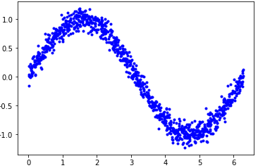
我们开始分训练集、验证集和测试集，如果不太懂这些概念的童鞋可以去康康我的博客哦《无废话的机器学习笔记》。

# We'll use 60% of our data for training and 20% for testing. The remaining 20%
# will be used for validation. Calculate the indices of each section.
TRAIN_SPLIT =  int(0.6 * SAMPLES)
TEST_SPLIT = int(0.2 * SAMPLES + TRAIN_SPLIT)
x_train, x_validate, x_test = np.split(x_values, [TRAIN_SPLIT, TEST_SPLIT])
y_train, y_validate, y_test = np.split(y_values, [TRAIN_SPLIT, TEST_SPLIT])

plt.plot(x_train, y_train, 'b.', label="Train")
plt.plot(x_validate, y_validate, 'y.', label="Validate")
plt.plot(x_test, y_test, 'r.', label="Test")
plt.legend()
plt.show()

模型1训练

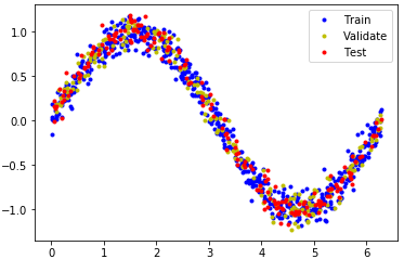
我们将建立一个模型，它将接受一个输入值(在本例中是x)，并使用它来预测一个数值输出值(x的正弦值)。这种类型的问题被称为回归。为了实现这一点，我们将创建一个简单的神经网络。它将使用神经元层来尝试学习训练数据下的任何模式，从而做出预测。首先，我们将定义两个层。第一层接受一个输入(我们的x值)，并通过16个神经元运行。基于这种输入，每个神经元会根据其内部状态(其权重和偏置值)被激活到一定程度。神经元的激活程度用数字表示。第一层的激活数将作为输入输入到第二层，也就是单个神经元。它会将自己的权重和偏差应用到这些输入，并计算自己的激活，它将作为我们的y值输出。下面单元格中的代码使用Keras (TensorFlow用于创建深度学习网络的高级API)定义了我们的模型。一旦网络被定义，我们将编译它，指定参数来决定它将如何训练。

模型1创建

# We'll use Keras to create a simple model architecture
from tensorflow.keras import layers
model_1 = tf.keras.Sequential()

# First layer takes a scalar input and feeds it through 16 "neurons". The
# neurons decide whether to activate based on the 'relu' activation function.
model_1.add(layers.Dense(16, activation='relu', input_shape=(1,)))

# Final layer is a single neuron, since we want to output a single value
model_1.add(layers.Dense(1))

# Compile the model using a standard optimizer and loss function for regression
model_1.compile(optimizer='rmsprop', loss='mse', metrics=['mae'])

# Print a summary of the model's architecture
model_1.summary()

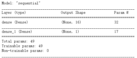
我们看到这个神经网络只有两层，弟中之弟哈哈，过于简单，来看看它的拟合效果怎样。

模型1训练

一旦我们定义了模型，我们就可以使用数据来训练它。训练包括向神经网络传递一个x值，检查网络的输出与期望的y值偏离多少，调整神经元的权值和偏差，以便下次输出更有可能是正确的。训练在完整数据集上多次运行这个过程，每次完整的运行都被称为一个epoch。训练中要运行的epoch数是我们可以设置的参数。在每个epoch期间，数据在网络中以多个批次运行。每个批处理，几个数据片段被传递到网络，产生输出值。这些输出的正确性是整体衡量的，网络的权重和偏差是相应调整的，每批一次。批处理大小也是我们可以设置的参数。下面单元格中的代码使用来自训练数据的x和y值来训练模型。它运行1000个epoch，每个批处理中有16条数据。我们还传入一些用于验证的数据。 没错，代码里就是一行的事。

# Train the model on our training data while validating on our validation set
history_1 = model_1.fit(x_train, y_train, epochs=1000, batch_size=16,
                    validation_data=(x_validate, y_validate))

检查训练指标

在训练过程中，模型的性能不断地根据我们的训练数据和我们早先留出的验证数据进行测量。训练产生一个数据日志，告诉我们模型的性能在训练过程中是如何变化的。

# Draw a graph of the loss, which is the distance between
# the predicted and actual values during training and validation.
loss = history_1.history['loss']
val_loss = history_1.history['val_loss']

epochs = range(1, len(loss) + 1)

plt.plot(epochs, loss, 'g.', label='Training loss')
plt.plot(epochs, val_loss, 'b', label='Validation loss')
plt.title('Training and validation loss')
plt.xlabel('Epochs')
plt.ylabel('Loss')
plt.legend()
plt.show()

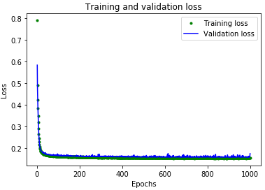
再靠近一点看数据：

# Exclude the first few epochs so the graph is easier to read
SKIP = 100

plt.plot(epochs[SKIP:], loss[SKIP:], 'g.', label='Training loss')
plt.plot(epochs[SKIP:], val_loss[SKIP:], 'b.', label='Validation loss')
plt.title('Training and validation loss')
plt.xlabel('Epochs')
plt.ylabel('Loss')
plt.legend()
plt.show()

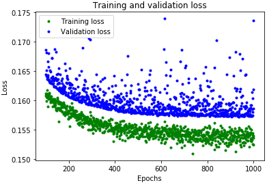
明显的过拟合，模型在测试集上表现不好，即只拟合了训练数据，真正应用就拉胯。

为了更深入地了解我们的模型的性能，我们可以绘制更多的数据。下面我们将绘制平均绝对误差MAE，这是另一种衡量网络预测距离实际数字有多远的方法:

# Draw a graph of mean absolute error, which is another way of
# measuring the amount of error in the prediction.
mae = history_1.history['mae']
val_mae = history_1.history['val_mae']

plt.plot(epochs[SKIP:], mae[SKIP:], 'g.', label='Training MAE')
plt.plot(epochs[SKIP:], val_mae[SKIP:], 'b.', label='Validation MAE')
plt.title('Training and validation mean absolute error')
plt.xlabel('Epochs')
plt.ylabel('MAE')
plt.legend()
plt.show()

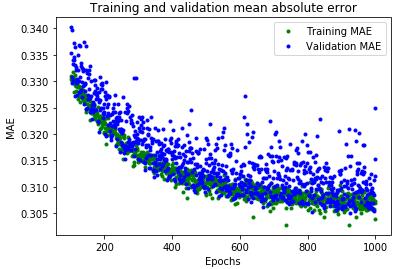
我们看到即使训练了1000次，误差也会有30%，太大了，我们画出拟合曲线看看有多离谱：

# Use the model to make predictions from our validation data
predictions = model_1.predict(x_train)

# Plot the predictions along with to the test data
plt.clf()
plt.title('Training data predicted vs actual values')
plt.plot(x_test, y_test, 'b.', label='Actual')
plt.plot(x_train, predictions, 'r.', label='Predicted')
plt.legend()
plt.show()

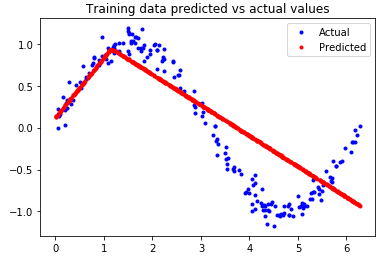
这张图清楚地表明，我们的网络已经学会了以一种非常有限的方式近似正弦函数。这些预测是高度线性的，只能非常粗略地符合数据。这种拟合的刚性表明，该模型没有足够的能力学习正弦波函数的全部复杂性，所以它只能以一种过于简单的方式近似它。把我们的模型做大，我们就能提高它的性能。

模型2训练

有了前面的“教训”，我们知道不能把神经网络设置太简单，至少要3层。

model_2 = tf.keras.Sequential()

# First layer takes a scalar input and feeds it through 16 "neurons". The
# neurons decide whether to activate based on the 'relu' activation function.
model_2.add(layers.Dense(16, activation='relu', input_shape=(1,)))

# The new second layer may help the network learn more complex representations
model_2.add(layers.Dense(16, activation='relu'))

# Final layer is a single neuron, since we want to output a single value
model_2.add(layers.Dense(1))

# Compile the model using a standard optimizer and loss function for regression
model_2.compile(optimizer='rmsprop', loss='mse', metrics=['mae'])

# Show a summary of the model
model_2.summary()

history_2 = model_2.fit(x_train, y_train, epochs=600, batch_size=16,
                    validation_data=(x_validate, y_validate))

# Draw a graph of the loss, which is the distance between
# the predicted and actual values during training and validation.
loss = history_2.history['loss']
val_loss = history_2.history['val_loss']

epochs = range(1, len(loss) + 1)

plt.plot(epochs, loss, 'g.', label='Training loss')
plt.plot(epochs, val_loss, 'b', label='Validation loss')
plt.title('Training and validation loss')
plt.xlabel('Epochs')
plt.ylabel('Loss')
plt.legend()
plt.show()

# Exclude the first few epochs so the graph is easier to read
SKIP = 80

plt.clf()

plt.plot(epochs[SKIP:], loss[SKIP:], 'g.', label='Training loss')
plt.plot(epochs[SKIP:], val_loss[SKIP:], 'b.', label='Validation loss')
plt.title('Training and validation loss')
plt.xlabel('Epochs')
plt.ylabel('Loss')
plt.legend()
plt.show()

plt.clf()

# Draw a graph of mean absolute error, which is another way of
# measuring the amount of error in the prediction.
mae = history_2.history['mae']
val_mae = history_2.history['val_mae']

plt.plot(epochs[SKIP:], mae[SKIP:], 'g.', label='Training MAE')
plt.plot(epochs[SKIP:], val_mae[SKIP:], 'b.', label='Validation MAE')
plt.title('Training and validation mean absolute error')
plt.xlabel('Epochs')
plt.ylabel('MAE')
plt.legend()
plt.show()

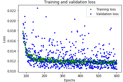
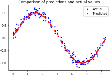
跟前面一样的步骤，我们可以看到误差很不错

# Calculate and print the loss on our test dataset
loss = model_2.evaluate(x_test, y_test)

# Make predictions based on our test dataset
predictions = model_2.predict(x_test)

# Graph the predictions against the actual values
plt.clf()
plt.title('Comparison of predictions and actual values')
plt.plot(x_test, y_test, 'b.', label='Actual')
plt.plot(x_test, predictions, 'r.', label='Predicted')
plt.legend()
plt.show()

 

模型导出（TensorFlow Lite）

模型已经被我们训练好了，但一般来说正常训练好的DL模型不能被部署到单片机上，因为太大了，我们将使用TensorFlow Lite转换器。转换器以一种特殊的、节省空间的格式输出文件，以便在内存受限的设备上使用。由于这个模型将部署在一个微控制器上，我们希望它尽可能小!量化是一种减小模型尺寸的技术。它降低了模型权值的精度，节省了内存。

# Convert the model to the TensorFlow Lite format without quantization
converter = tf.lite.TFLiteConverter.from_keras_model(model_2)
tflite_model = converter.convert()

# Save the model to disk
open("sine_model.tflite", "wb").write(tflite_model)

# Convert the model to the TensorFlow Lite format with quantization
converter = tf.lite.TFLiteConverter.from_keras_model(model_2)
# Indicate that we want to perform the default optimizations,
# which includes quantization
converter.optimizations = [tf.lite.Optimize.DEFAULT]
# Define a generator function that provides our test data's x values
# as a representative dataset, and tell the converter to use it
def representative_dataset_generator():
  for value in x_test:
    # Each scalar value must be inside of a 2D array that is wrapped in a list
    yield [np.array(value, dtype=np.float32, ndmin=2)]
converter.representative_dataset = representative_dataset_generator
# Convert the model
tflite_model = converter.convert()

# Save the model to disk
open("sine_model_quantized.tflite", "wb").write(tflite_model)

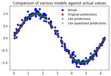
模型转化后我们可能怀疑它的准确性会不会下降，答案是不会的，误差不会差多少，可以试试下面的代码看看转换后的模型与原本的模型对比，发现差不多，很准确。

# Instantiate an interpreter for each model
sine_model = tf.lite.Interpreter('sine_model.tflite')
sine_model_quantized = tf.lite.Interpreter('sine_model_quantized.tflite')

# Allocate memory for each model
sine_model.allocate_tensors()
sine_model_quantized.allocate_tensors()

# Get indexes of the input and output tensors
sine_model_input_index = sine_model.get_input_details()[0]["index"]
sine_model_output_index = sine_model.get_output_details()[0]["index"]
sine_model_quantized_input_index = sine_model_quantized.get_input_details()[0]["index"]
sine_model_quantized_output_index = sine_model_quantized.get_output_details()[0]["index"]

# Create arrays to store the results
sine_model_predictions = []
sine_model_quantized_predictions = []

# Run each model's interpreter for each value and store the results in arrays
for x_value in x_test:
  # Create a 2D tensor wrapping the current x value
  x_value_tensor = tf.convert_to_tensor([[x_value]], dtype=np.float32)
  # Write the value to the input tensor
  sine_model.set_tensor(sine_model_input_index, x_value_tensor)
  # Run inference
  sine_model.invoke()
  # Read the prediction from the output tensor
  sine_model_predictions.append(
      sine_model.get_tensor(sine_model_output_index)[0])
  # Do the same for the quantized model
  sine_model_quantized.set_tensor(sine_model_quantized_input_index, x_value_tensor)
  sine_model_quantized.invoke()
  sine_model_quantized_predictions.append(
      sine_model_quantized.get_tensor(sine_model_quantized_output_index)[0])


# See how they line up with the data
plt.clf()
plt.title('Comparison of various models against actual values')
plt.plot(x_test, y_test, 'bo', label='Actual')
plt.plot(x_test, predictions, 'ro', label='Original predictions')
plt.plot(x_test, sine_model_predictions, 'bx', label='Lite predictions')
plt.plot(x_test, sine_model_quantized_predictions, 'gx', label='Lite quantized predictions')
plt.legend()
plt.show()

为微控制器使用TensorFlow Lite准备模型的最后一步是将其转换为C（或h）源文件。为此，我们可以使用一个名为xxd的命令行实用程序。下面的单元格在量化模型上运行xxd并打印输出:

# Install xxd if it is not available
!apt-get -qq install xxd
# Save the file as a C source file
!xxd -i sine_model_quantized.tflite > sine_model_quantized.cc
# Print the source file
!cat sine_model_quantized.cc

这样我们整个模型就被导出为c文件！！！搞嵌入式的应该很熟悉了！我们也可以导出为.h文件，在arduino里include一下就行，很方便。

 

模型部署、功能编写

有了.c文件，我们开始搞单片机，打开arduino，官方的代码是用arduino nano ble 33，但这个板子太贵了，10几块的esp32完全可以驾驭TinyML，所以我们用esp32。（STM32也完全可以的，不过没有arduino方便，有空我也会出个基于stm32的TinyML教程）

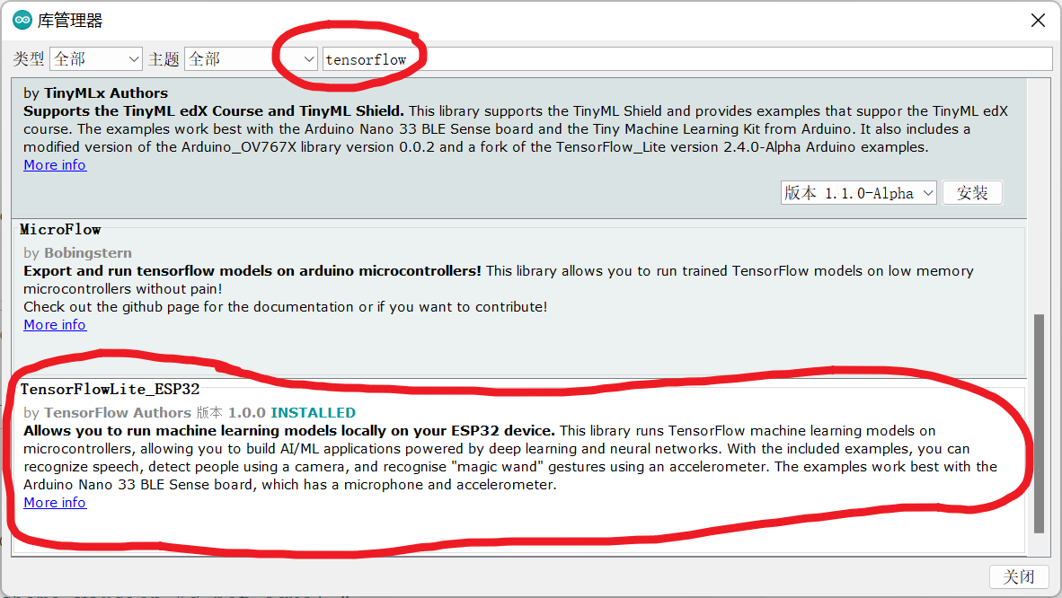
下载这个库，然后找到示例里面的hello world，点开。（默认大家已经装了esp32的库了，如果没有在库管理器里搜esp32安装就行）

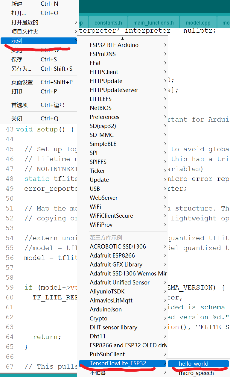
这个代码就是根据官方写的而改编的esp32版本，不过还有地方要改，点击它的output_handler.cpp文件，然后将其替换为下面的代码：

#include "output_handler.h"

#include "Arduino.h"
#include "constants.h"

int led = 2;
bool initialized = false;

void HandleOutput(tflite::ErrorReporter* error_reporter, float x_value,
                  float y_value) {

      // Do this only once
        if (!initialized) {
          ledcSetup(0, 5000, 13);
          // Set the LED pin to output
          ledcAttachPin(led, 0);
          //pinMode(led, OUTPUT);
          initialized = true;
        }
      
        // Calculate the brightness of the LED such that y=-1 is fully off
        // and y=1 is fully on. The LED's brightness can range from 0-255.
        int brightness = (int)(127.5f * (y_value + 1));
      
        // Set the brightness of the LED. If the specified pin does not support PWM,
        // this will result in the LED being on when y > 127, off otherwise.
        //analogWrite(led, brightness);

          uint32_t duty = (8191 / 255) * min(brightness, 255);
          ledcWrite(0, duty);

          //delay(30);

        
      
        // Log the current brightness value for display in the Arduino plotter
        TF_LITE_REPORT_ERROR(error_reporter, "%d\n", brightness);

                    
//  // Log the current X and Y values
//  TF_LITE_REPORT_ERROR(error_reporter, "x_value: %f, y_value: %f\n",
//                       static_cast<double>(x_value),
//                       static_cast<double>(y_value));
}

还有一个小地方，constans.cpp这个文件里面的kInferencesPerCycle改为200左右，不然灯闪得太快了。
上面的代码的model.cpp里面那一大坨数字就是训练好的模型，我们自己训练的跟它差不多，如果你想用自己的，把自己转换好的模型粘贴进去就好，记得把长度也填在最后一行。
ok，编译，你就会看到板子上的灯以一个正弦波的节奏在呼吸，恭喜你成功地实现了嵌入式ML、边缘AI、TinyML。
CV和NLP方面的有趣的TinyML应用现在也有了很多，我有空都出些教程。