MOPSO 多目标粒子群算法

1、算法简介

多目标粒子群（MOPSO）算法是由CarlosA. Coello Coello等人在2004年提出，目的是将原来只能用在单目标上的粒子群算法（PSO）应用于多目标上。

1.1、相关知识点

支配（Dominance ) :在多目标优化问题中，如果个体p至少有一个目标比个体q好，而且个体p的所有目标都不比q差；那么称个体p支配个体q

序值(Rank):如果p支配q，那么p的序值比q低;如果p和q互不支配，那么p和q有相同的序值

拥挤距离(Crowding Distance):表示个体之间的拥挤程度，测量相同序值个体之间的距离。

帕累托（Pareto）：https://blog.csdn.net/m0_59838738/article/details/121588306

粒子群算法（PSO）：承接我的博客

2、算法描述

2.1、PSO 对比 MOPSO

PSO:

|

MOPSO：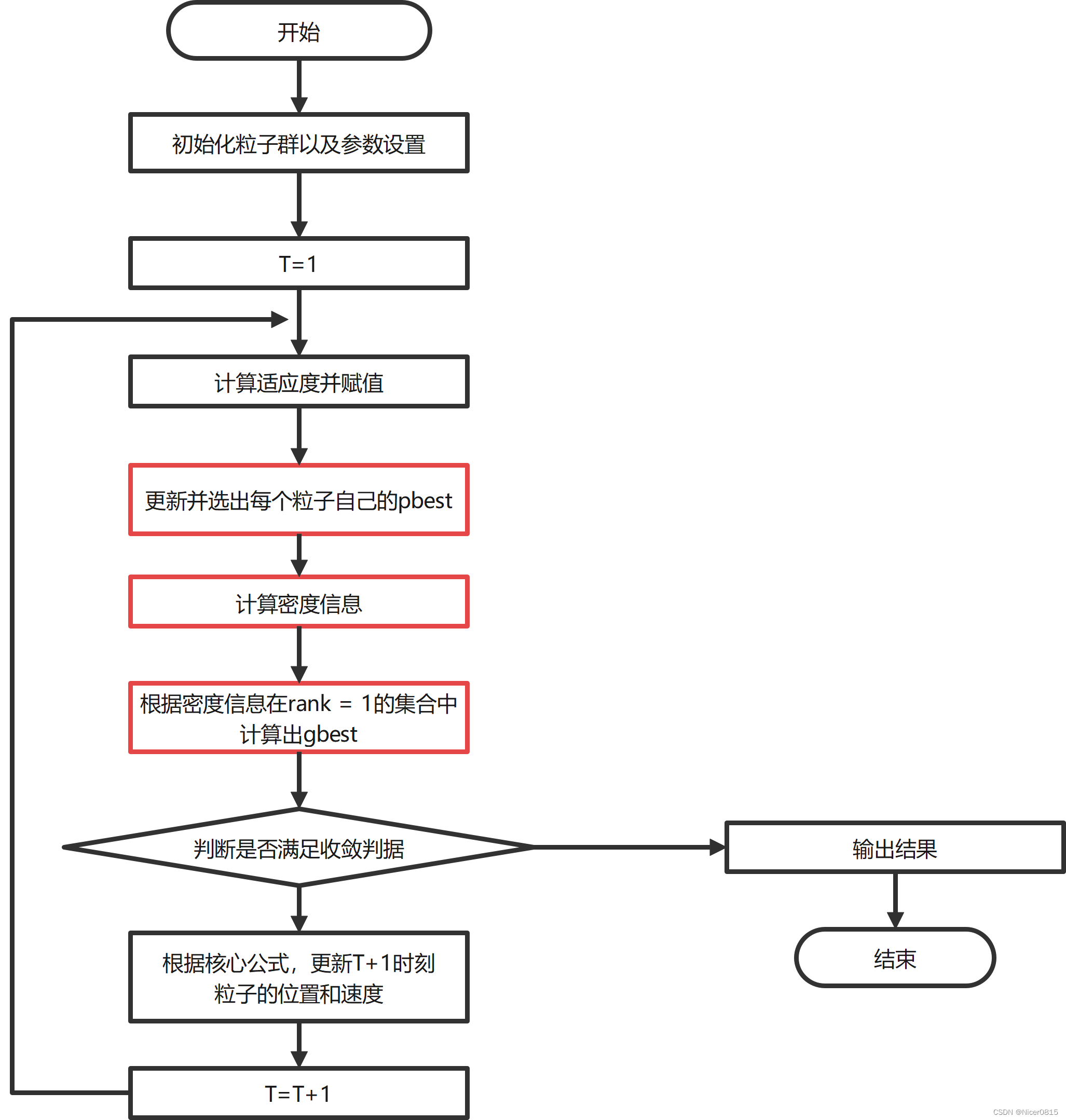

MOPSO注：

• 根据pareto支配原则，计算得到Archive集(存放当前的非劣解)计算局部最优pbest
• 计算Archive集中的拥挤度在Archive集选择全局最优gbest
• 更新粒子的速度和位置，并计算适应值更新Archive集（需注意防止溢出)

结论：可以看出PSO和MOPSO的大框架一致，MOPSO只是根据多目标问题改进了PSO中的pbest和gbest的选取方法

• pbest的选取：
  • 单目标问题中，PSO可以根据适应度直接找出该粒子历史最好的位置；
  • 多目标问题中，MOPSO找出该粒子历史最好的位置（保存于该粒子结构体的一个属性中）；
    • 如果在更新当前粒子的历史最好位置发现当前位置与历史最佳互不支配，0.5概率随机选一个；
• gbest的选取
  • 单目标问题中，PSO可以根据适应度直接找出当前最好的粒子；
  • 多目标问题中，MOPSO根据Pareto找出当前最好的粒子集合，至于最后精确到哪个粒子，找到最不拥挤的那个粒子；

2.2、密度的计算

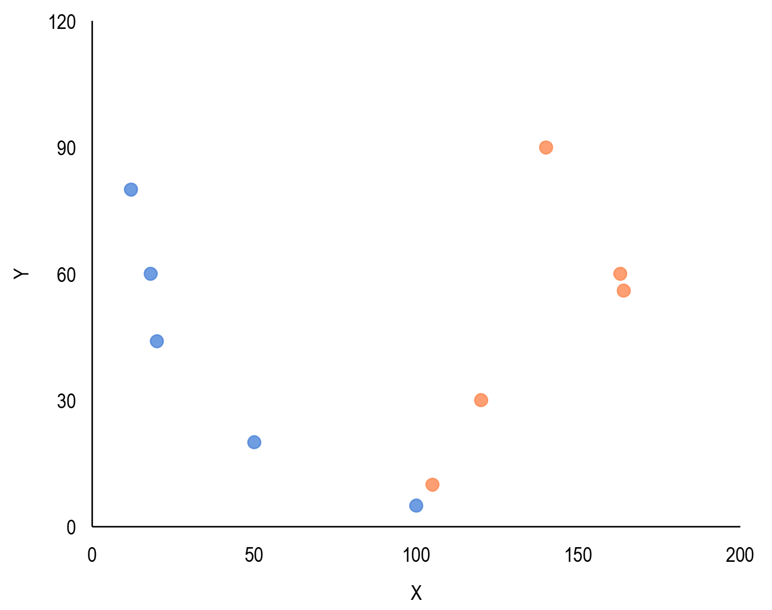
与我的NSGA-II的博客的2.3拥挤距离类似，这里采用了网格法：

把目标空间用网格等分成小区域，以每个区域中包含的粒子数作为粒子的密度信息。粒子所在网格中包含的粒子数越多，其密度值越大，反之越小。

以二维目标空间最小化优化问题为例，密度信息估计算法的具体实现过程如下：

（1）假设我们现在得到一代种群粒子如下：

（2）根据输入的粒子坐标，可以确定每个维度的最大最小值，计算成坐标保存：即图示的两个黑点坐标

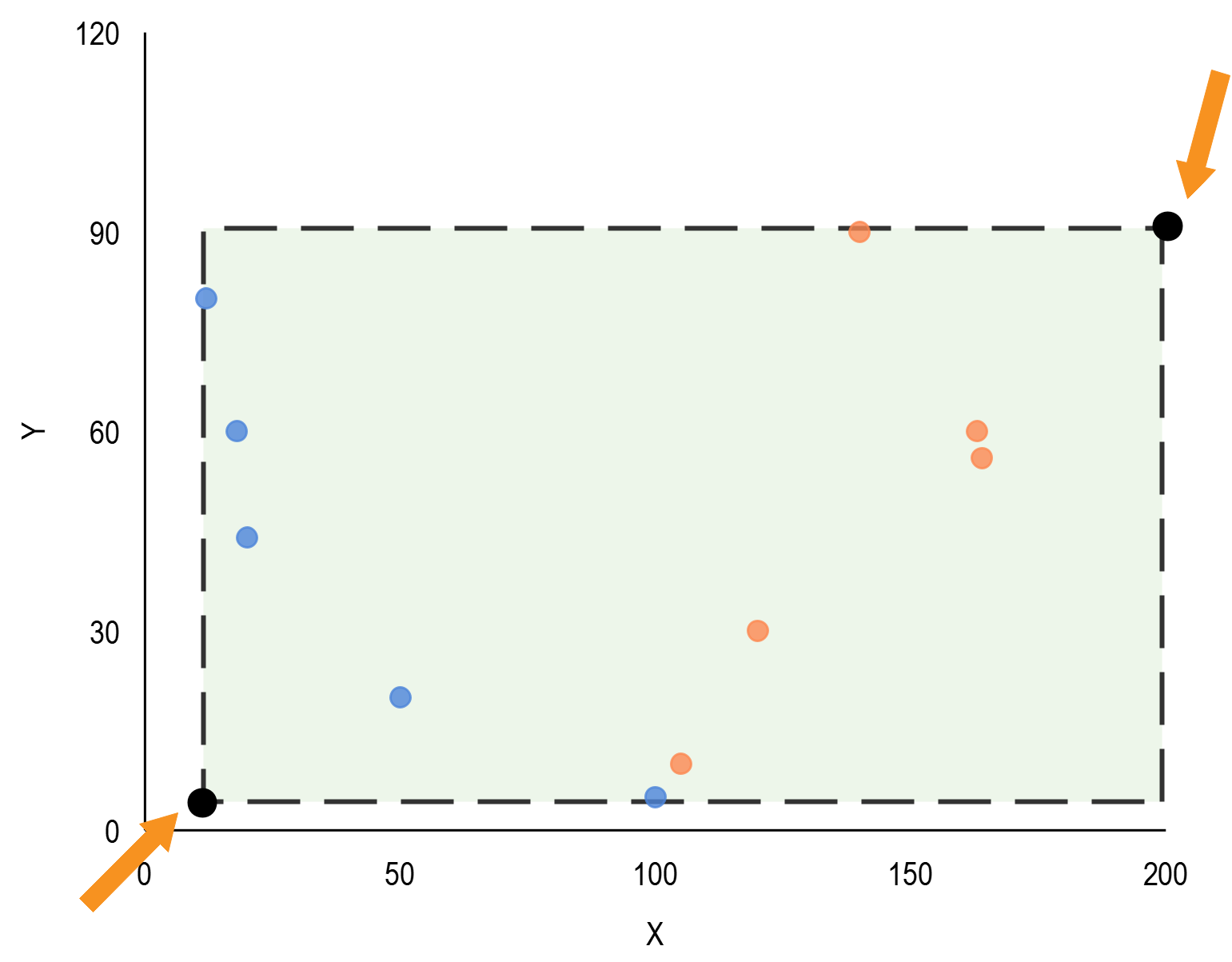
（3）划分格子，一般情况下我们会对边界进行一次膨胀，然后根据nGrid参数进行每个维度的等额划分：假设我们设置了参数nGrid = 3即每个维度划分3个网格

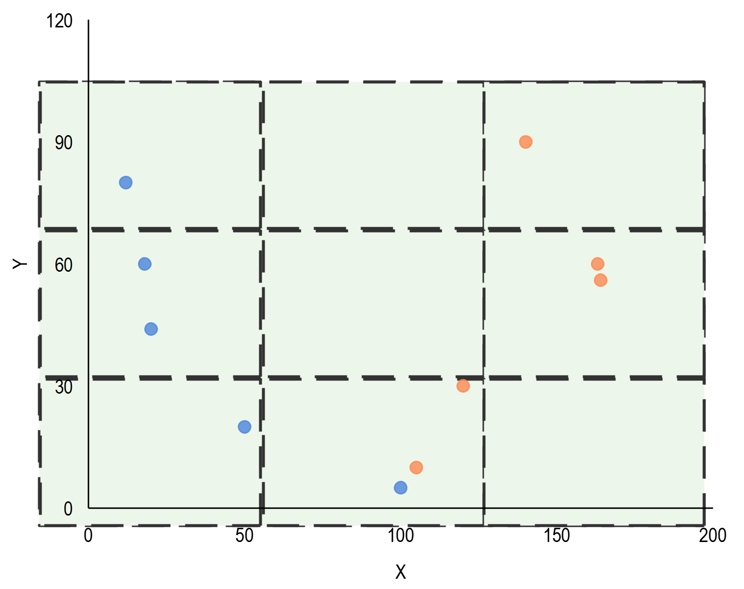
（4）存储格子信息，如上下界，格子编号等。然后根据粒子坐标即可统计格子内的粒子数。

3、算法流程图

4、代码实操

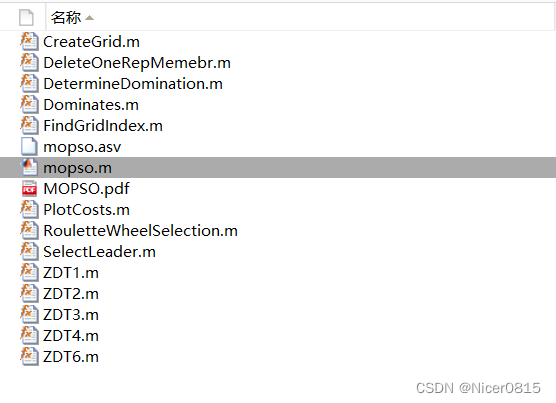
下面展示ZDT1~4系列问题的求解代码

4.1、代码

（1）文件目录：

（2）网格创建函数

function Grid = CreateGrid(pop, nGrid, alpha)

    c = [pop.Cost];

    %M = min(A,[],dim) 返回维度 dim 上的最小元素。例如，如果 A 为矩阵，则 min(A,[],2) 是包含每一行的最小值的列向量。
    cmin = min(c, [], 2);
    cmax = max(c, [], 2);
    
    dc = cmax-cmin;

    %网格边界外扩
    cmin = cmin-alpha*dc;
    cmax = cmax+alpha*dc;
    
    nObj = size(c, 1);
    
    %网格上下界
    empty_grid.LB = [];
    empty_grid.UB = [];
    Grid = repmat(empty_grid, nObj, 1);
    
    for j = 1:nObj
        %y = linspace(x1,x2,n) 生成 n 个点。这些点的间距为 (x2-x1)/(n-1)。
        cj = linspace(cmin(j), cmax(j), nGrid+1);       % nGrid是设置好的参数
        
        Grid(j).LB = [-inf cj];
        Grid(j).UB = [cj +inf];
        
    end

end

（3）支配计算函数1

function pop = DetermineDomination(pop)

    nPop = numel(pop);
    
    for i = 1:nPop
        pop(i).IsDominated = false;
    end
    
    for i = 1:nPop-1
        for j = i+1:nPop
            % b = all(x <= y) && any(x<y);
            if Dominates(pop(i), pop(j))  %i支配j
               pop(j).IsDominated = true;
            end
            
            if Dominates(pop(j), pop(i))
               pop(i).IsDominated = true;
            end
            % 有重复比对的过程
        end
    end

end

（4）支配计算函数2

function b = Dominates(x, y)

    if isstruct(x)
        x = x.Cost;
    end
    
    if isstruct(y)
        y = y.Cost;
    end

    b = all(x <= y) && any(x<y);

end

（5）网格查找函数，遍历粒子，统计网格

function particle = FindGridIndex(particle, Grid)

    nObj = numel(particle.Cost);
    
    nGrid = numel(Grid(1).LB);
    
    particle.GridSubIndex = zeros(1, nObj);
    
    for j = 1:nObj
        
        particle.GridSubIndex(j) = ...
            find(particle.Cost(j)<Grid(j).UB, 1, 'first');
        
    end

    particle.GridIndex = particle.GridSubIndex(1);
    for j = 2:nObj
        particle.GridIndex = particle.GridIndex-1;
        particle.GridIndex = nGrid*particle.GridIndex;
        particle.GridIndex = particle.GridIndex+particle.GridSubIndex(j);
    end
    
end

（6）轮盘选择函数

function i = RouletteWheelSelection(P)

    r = rand;
    
    C = cumsum(P);
    
    i = find(r <= C, 1, 'first');

end

（7）gbest选择函数，选一个当全局最优

function leader = SelectLeader(rep, beta)

    % Grid Index of All Repository Members
    GI = [rep.GridIndex];
    
    % Occupied Cells
    OC = unique(GI);
    
    % Number of Particles in Occupied Cells
    N = zeros(size(OC));
    for k = 1:numel(OC)
        N(k) = numel(find(GI == OC(k)));
    end
    
    % Selection Probabilities
    P = exp(-beta*N);
    P = P/sum(P);
    
    % Selected Cell Index 轮盘选择
    sci = RouletteWheelSelection(P);
    
    % Selected Cell
    sc = OC(sci);
    
    % Selected Cell Members
    SCM = find(GI == sc);
    

    % 网格里可能还有多个粒子 再随机选一个
    % Selected Member Index
    smi = randi([1 numel(SCM)]);
    
    % Selected Member
    sm = SCM(smi);
    
    % Leader
    leader = rep(sm);

end

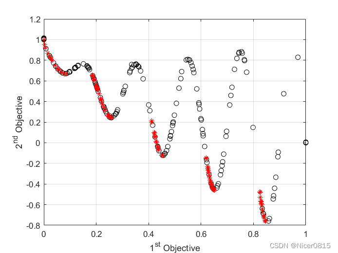
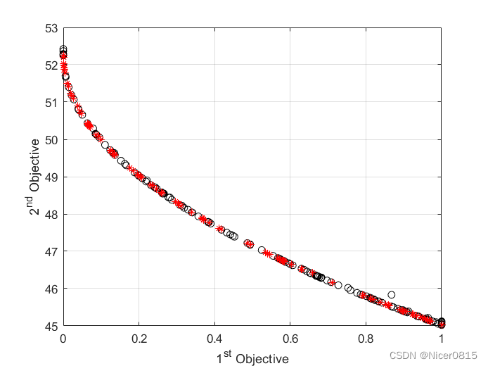
（8）绘图函数

function PlotCosts(pop, rep)

    pop_costs = [pop.Cost];
    plot(pop_costs(1, :), pop_costs(2, :), 'ko');
    hold on;
    
    rep_costs = [rep.Cost];
    plot(rep_costs(1, :), rep_costs(2, :), 'r*');
    
    xlabel('1^{st} Objective');
    ylabel('2^{nd} Objective');
    
    grid on;
    
    hold off;

end

（9）ZDT1~4

function z = ZDT1(x)

    n = numel(x);

    f1 = x(1);
    
    g = 1+9/(n-1)*sum(x(2:end));
    
    h = 1-sqrt(f1/g);
    
    f2 = g*h;
    
    z = [f1
       f2];

end

function z = ZDT2(x)

    n = numel(x);

    f1 = x(1);
    
    g = 1+9/(n-1)*sum(x(2:end));
    
    h = 1-(f1/g)^2;
    
    f2 = g*h;
    
    z = [f1
       f2];

end
function z = ZDT3(x)

    n = numel(x);

    f1 = x(1);
    
    g = 1+9/(n-1)*sum(x(2:end));
    
    %h = 1-(f1/g)^2;  % ZDT2与3的不同之处
    h = (1-(f1/g)^0.5-(f1/g)*sin(10*pi*f1));
    
    f2 = g*h;
    
    z = [f1
       f2];

end
function z = ZDT4(x)

    n = numel(x);

    f1 = x(1);

    sum=0;
    for i=2:n
        sum = sum+(x(i)^2-10*cos(4*pi*x(i)));
    end

    g = 1+9*10+sum;

    h = (1-(f1/g)^0.5);
    
    f2 = g*h;
    
    z = [f1
       f2];

end

（10）主函数

clc;
clear;
close all;

%% Problem Definition

CostFunction = @(x) ZDT3(x);      % Cost Function

nVar = 5;             % 5个决策变量

VarSize = [1 nVar];   % Size of Decision Variables Matrix

VarMin = 0;          % Lower Bound of Variables
VarMax = 1;          % Upper Bound of Variables


%% MOPSO Parameters

MaxIt = 200;           % 迭代次数

nPop = 200;            % 种群大小

nRep = 100;            % 精英库

w = 0.5;              % 惯性权重
wdamp = 0.99;         % 惯性权重的衰减因子（阻尼）
c1 = 1;               % 个体学习因子
c2 = 2;               % 全局学习因子

nGrid = 7;            % 每个维度的网格数
alpha = 0.1;          % 膨胀率  网格边界外扩大小的因子

beta = 2;             % Leader Selection Pressure
gamma = 2;            % Deletion Selection Pressure

mu = 0.1;             % 变异率

%% Initialization

empty_particle.Position = [];
empty_particle.Velocity = [];
empty_particle.Cost = [];
empty_particle.Best.Position = [];
empty_particle.Best.Cost = [];
empty_particle.IsDominated = [];
empty_particle.GridIndex = [];
empty_particle.GridSubIndex = [];

pop = repmat(empty_particle, nPop, 1);

for i = 1:nPop
    
    pop(i).Position = unifrnd(VarMin, VarMax, VarSize);
    
    pop(i).Velocity = zeros(VarSize);
    
    pop(i).Cost = CostFunction(pop(i).Position);  % CostFunction = @(x) ZDT(x); 适应度
    
    
    % Update Personal Best
    pop(i).Best.Position = pop(i).Position;
    pop(i).Best.Cost = pop(i).Cost;
    
end

% 计算种群的支配情况
pop = DetermineDomination(pop);

% 取出没有被支配的pop元素，存放到rep
rep = pop(~[pop.IsDominated]);

% 根据粒子分布画出网格
Grid = CreateGrid(rep, nGrid, alpha);

% 根据粒子位置确定所处网格
for i = 1:numel(rep)
    rep(i) = FindGridIndex(rep(i), Grid);
end


%% MOPSO Main Loop

for it = 1:MaxIt
    
    for i = 1:nPop
        
        gbest = SelectLeader(rep, beta);
        
        pop(i).Velocity = w*pop(i).Velocity ...
            +c1*rand(VarSize).*(pop(i).Best.Position-pop(i).Position) ...
            +c2*rand(VarSize).*(gbest.Position-pop(i).Position);
        
        pop(i).Position = pop(i).Position + pop(i).Velocity;
        
        pop(i).Position = max(pop(i).Position, VarMin);
        pop(i).Position = min(pop(i).Position, VarMax);
        
        pop(i).Cost = CostFunction(pop(i).Position);
        
        % 更新i粒子历史最优
        if Dominates(pop(i), pop(i).Best)
            pop(i).Best.Position = pop(i).Position;
            pop(i).Best.Cost = pop(i).Cost;
            
        elseif Dominates(pop(i).Best, pop(i))
            % Do Nothing
            
        else
            if rand<0.5
                pop(i).Best.Position = pop(i).Position;
                pop(i).Best.Cost = pop(i).Cost;
            end
        end
        
    end
    
    % Add Non-Dominated Particles to REPOSITORY
    % 把更新后的rank = 1的粒子再加到rep
    rep = [rep
         pop(~[pop.IsDominated])]; %#ok
    
    % Determine Domination of New Resository Members
    % 上一代的Non-Dominated粒子和当前代的粒子进行支配判断
    rep = DetermineDomination(rep);
    
    % Keep only Non-Dminated Memebrs in the Repository
    rep = rep(~[rep.IsDominated]);
    
    % Update Grid
    Grid = CreateGrid(rep, nGrid, alpha);

    % Update Grid Indices
    for i = 1:numel(rep)
        rep(i) = FindGridIndex(rep(i), Grid);
    end
    
    % Check if Repository is Full
    if numel(rep)>nRep
        
        Extra = numel(rep)-nRep;
        for e = 1:Extra
            % 轮盘删一个，类似选取pbest的流程
            rep = DeleteOneRepMemebr(rep, gamma);
        end
        
    end
    
    % Plot Costs
    figure(1);
    PlotCosts(pop, rep);
    pause(0.01);
    
    % Show Iteration Information
    disp(['Iteration ' num2str(it) ': Number of Rep Members = ' num2str(numel(rep))]);
    
    % Damping Inertia Weight
    w = w*wdamp;
    
end

之前漏掉的函数DeleteOneRepMemebr【sorry】

function rep = DeleteOneRepMemebr(rep, gamma)

    % Grid Index of All Repository Members
    GI = [rep.GridIndex];
    
    % Occupied Cells
    OC = unique(GI);
    
    % Number of Particles in Occupied Cells
    N = zeros(size(OC));
    for k = 1:numel(OC)
        N(k) = numel(find(GI == OC(k)));
    end
    
    % Selection Probabilities
    P = exp(gamma*N);
    P = P/sum(P);
    
    % Selected Cell Index
    sci = RouletteWheelSelection(P);
    
    % Selected Cell
    sc = OC(sci);
    
    % Selected Cell Members
    SCM = find(GI == sc);
    
    % Selected Member Index
    smi = randi([1 numel(SCM)]);
    
    % Selected Member
    sm = SCM(smi);
    
    % Delete Selected Member
    rep(sm) = [];

end

4.2、ZDT1~4的运行结果

|

|
|