目录

1 前言

2 方法综述

2.1 时频分析法

2.1.1 短时傅里叶变换

2.1.2 小波变换

2.1.3 希尔伯特-黄变换

2.2 图像编码方法

2.2.1 格兰姆角场

2.2.2 马尔可夫转移场

2.2.3 递归图

2.2.4 图形差分场

2.2.5 相对位置矩阵

3 应用研究现状

4 方法仿真与分析

5 总结与分析

6 参考文献

---

【声明：本文禁止被转载和抄袭】

【若觉文章质量良好且有用，请别忘了点赞收藏加关注，这将是我继续分享的动力，万分感谢！】

1 前言

时间序列是指按时间的顺序关于事件变化发展的过程记录，它保存了观测数据的时间结构性。因此时间序列常常被当成一个整体进行研究分析，而不是一个个独立的数值。许多工程领域的数据都以时间序列的形式存在，如医学上的心率记录、心电图，公司的财务报表，股票市场价格，交通拥堵指数，还有流行病的传播情况等，这些都是典型的时间序列数据。时间序列有数据量大、维度高、实时更新等特点，针对时间序列数据分析的目的主要有预测、聚类、分类（包括异常检测）、关联分析等。在这些任务中，时间序列分类问题是现有相关研究中备受关注的[2]。

现如今，随着时间序列数据的不断增加，分析目的的不断深入和拓展，使用传统的方法提高时间序列分类问题的精度越来越困难。然而，近年来由于数据量和计算量的不断增加，深度学习快速发展并迅速成为数据研究的重要法宝。其中，卷积神经网络（CNN）是发展最快、技术相对最成熟、且应用最成功的深度学习模型。从经典的LeNet[3]、AlexNet[4]、ResNet[5]到EfficentNet[6]，CNN网络结构推陈出新，不断发展。CNN通过共享权重，一方面大幅度减少模型大小，使得网络优化快速迭代，另一方面降低了过拟合风险，有更好的泛化能力。这些使得CNN在多个领域中成功应用，并取得了巨大的效果，尤其在图像领域的分类任务。

考虑到时间序列分类任务面对的困难和CNN在图像分类任务中取得的巨大成功，相关领域的研究者提出了这样的观点：将一维时间序列数据转化为二维图像，把时间序列分类任务转化为图像分类任务，再用CNN模型进行训练学习。从宏观的角度分析，时间序列的分类任务与图像领域的分类任务具有一定的相似性，都是从数据中提取关键特征，再根据特征进行分类。正是这种相似性，促使一些新的研究出现，比如将时间序列数据转化为二维图像的方法研究、将转为方法实际应用到相关领域的研究等等。本文将系统综述时间序列数据转化为二维图像的方法以及其相关应用，最后采用案例研究分析各个方法的优劣。

2 方法综述

在计算机中图像可以用矩阵的形式表示。因此，将时间序列转化为图像等价于将时间序列转化为矩阵。根据这个原则，如表1所示，本论文整理了两大类方法：第一大类为时频分析方法，将时间序列作为信号分析对象，采用时频分析方法分析求解其时频图，主要有短时傅里叶变换[7]，小波变换[8]，希尔伯特-黄变换[9]；第二大类为图像编码方法，这一大类方法指的是通过其他方法对时间序列进行图像编码，主要有格兰姆角场[10]，马尔可夫转移场[10]，递归图[11]，图形差分场[12]，相对位置矩阵[13]。下面详细介绍各种方法。

表1：时间序列转二维图像方法归类

归类	方法	简单描述
时频分析方法	短时傅里叶变换	选择适当的窗函数；计算窗口内信号的相频信息；推动窗口，得到信号的时频图。
	小波变换	构造一个快速衰减的母小波；通过缩放和平移得到子小波；进行参数匹配和叠加拟合信号。
	希尔伯特-黄变换	通过经验模态分解信号得到有限数量的模态函数；对IMF分量进行希尔伯特变换，得到瞬时频率。
图像编码方法	格兰姆角场	通过空间变换来消除时间序列噪声；采用向量内积来保存时间信息。
	马尔可夫转移场	将时间顺序看成是马尔可夫过程；分成Q个分位箱，构造马尔可夫转移矩阵，生成马尔可夫转移场。
	递归图	将时域空间变换位相空间，即每个点变换成相空间中的对应状态；计算状态之间的距离，从而得到相应的图像特征。
	图形差分法	通过截取图形不同长度，进行差分等处理，构造图形差分场；保留序列熵(复杂性测量、动态系统特征)
	相对位置矩阵	先进行z-分值标准化，采用PAA进行降维，计算每两个时间戳之间的相对大小关系，最后转换为灰度值矩阵。

2.1 时频分析法

将时间序列看成是一个频率和相位随时间变化的信号，根据时频分析方法，可将时间序列数据转换成时频图，其主要方法有短时傅里叶变换、小波变换、希尔伯特-黄变换。

2.1.1 短时傅里叶变换

见：将时间序列转成图像——短时傅里叶方法 Matlab实现_vm-1215的博客-CSDN博客

2.1.2 小波变换

见：将时间序列转成图像——小波变换方法 Matlab实现_vm-1215的博客-CSDN博客

2.1.3 希尔伯特-黄变换

见：将时间序列转成图像——希尔伯特-黄变换方法 Matlab实现_vm-1215的博客-CSDN博客

2.2 图像编码方法

2.2.1 格兰姆角场

见：将时间序列转成图像——格拉姆角场方法 Matlab实现_vm-1215的博客-CSDN博客

2.2.2 马尔可夫转移场

 见：将时间序列转成图像——马尔可夫转移场方法 Matlab实现_vm-1215的博客-CSDN博客

2.2.3 递归图

见：将时间序列转成图像——递归图方法 Matlab实现_vm-1215的博客-CSDN博客

2.2.4 图形差分场

见：将时间序列转成图像——图形差分场方法 Matlab实现_vm-1215的博客-CSDN博客

2.2.5 相对位置矩阵

见：将时间序列转成图像——相对位置矩阵方法 Matlab实现_vm-1215的博客-CSDN博客

3 应用研究现状

表2：时间序列转二维图像的应用研究

方法	文献	应用场景	主要工作
格拉姆角场	[16]	交通事件检测	采用分段聚合近似(PAA)将车辆速度时间序列数据不同长度转化为同一长度，通过格拉姆角场编码为图像，放入CNN模型中进行训练和检测。
	[17]	输电线路故障检测和分类	采用离散小波变换对故障电压和电流信号进行去噪处理，得到时间序列数据，通过格拉姆角场编码为图像，采用提出的SAT-CNN模型进行训练检测。
	[18]	基于可穿戴传感器的人类活动识别	将传感器数据的时间序列通过格拉姆角场编码为双通道图像，利用CNN模型进行训练识别；采用融合残差网络融合训练异构数据。
	[19]	输送机电机的预测性维护	采用主成分分析方法将多变量时间序列减少到最多两个通道，通过格拉姆角场编码为图像，采用带有PReLU的CNN模型进行预测维护。
	[20]	动作识别	采用格拉姆角场将可佩戴传感器的一维时间序列信号转换为二维图像，然后提出语义感知自适应知识蒸馏网络，提升视觉传感器模态中的动作识别。
	[21]	表面肌电信号分类	过分段聚合近似(PAA)和格拉姆角场将表面肌电信号编码为图像，引入胶囊网络和卷积神经网络进行特征提取和融合，实现不同条件下的手势识别。
	[22]	金融预测	通过格拉姆角场将与标准普尔500指数期货相关的时间序列编码为二维图像，采用简化的VGG网络作为识别网络，输出交易策略（做多、做空、持有）。
马尔可夫转移场	[23]	住宅建筑能耗异常识别	首先将能耗数据进行分割，然后计算基本统计、执行频谱分析或应用信号处理技术进行特征提取，再通过马尔可夫转移场将特征编码为二维图像，采用一类支持向量机完成分类任务。
递归图	[24]	时间序列预测	首先将时间序列转换成递归图，然后使用计算机视觉算法从递归图中提取局部特征，用于预测模型平均。
	[25]	旋转机械状态监测	将三相电流信号的时间序列数据编码为递归图，然后分类器从纹理图像中自动学习特征以分类电机的故障状态。
图形差分场	[26]	机械故障检测	在故障工业机器调查和检查的声音数据集(MIMII数据集)中，采用图形差分场将时间序列编码为图像，再用全连接网络进行识别分类。
相对位置矩阵	[13]	时间序列分类	采用相对位置矩阵将时间序列数据表示为二维图像，基于VGG的改进模型进行分类。

时间序列数据转化为二维图像的目的，是为了更好的提取特征，从而取得更佳的表现效果。如表2所示，是近年来相关研究者在不同领域中应用该类方法的研究现状，主要介绍各项研究的研究场景、使用的方法以及主要工作。在各项研究中，该类方法进行实际应用主要有以下两个问题：

1. 分析任务多样，如分类、异常检测、预测等，其需要分析的数据长度可能长度不一，则转化后的图像大小可能也不一样。
2. 以时间序列数据形式存在的场景多样，比如机械状态监控、金融、交通流量等，因此其属性可能有一种，也可能有多种。

针对以上问题，主要有以下解决方案：

1. 直接应用VS数据预处理：有的数据本身长度同一，可以直接应用时间序列转二维图像的方法；而有的数据长度不一样，则可以用分段聚合近似等方法同一化数据长度，再进行图像转化。此外，有的数据本身存在很大的噪声，或者需要提取出其他有代表性的时序数据特征，这些情况都可以在应用该类方法前进行数据预处理。

   类别	文献
   直接应用	[18]、[19]、[20]、[22]、[24]、[25]、[26]
   数据预处理	[16]、[17]、[21]、[23]、[13]

2. 单通道VS多通道：时间序列数据的每一种属性都可以通过图像化转化为一张图，作为整体转化后的图当中的一个通道。因而如果只有一种属性，其转化后为一张单通道的图；如果有多种属性，则转化为一张多通道的图。此外，如果属性种类过多且属性相关性较大，也可以通过主成分分析方法进行降维。

   类别	文献
   单通道	[16]、[17]、[20]、[21]、[22]、[23]、[24]、[25]、[26]、[13]
   多通道	[18]、[19]

4 方法仿真与分析

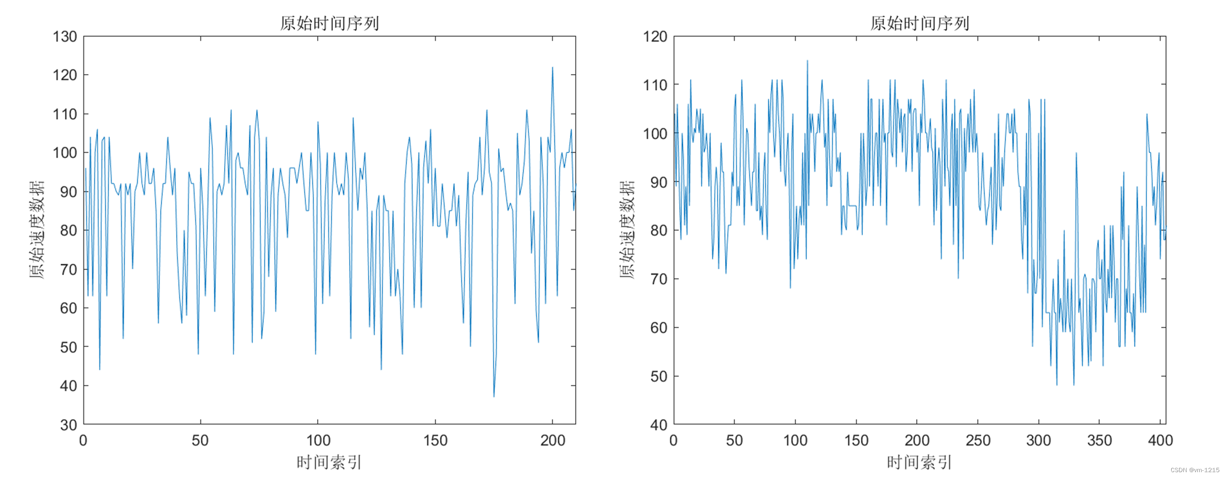
为了进一步分析不同时间序列转图像方法的性能，这里对所有方法进行逐一实现。如图1所示有两条时间序列数据，该数据为广州机场高速公路上某一路段某一段时间内的汽车速度数据，左图为正常情况下的速度数据，右图为发生异常事件情况下的速度数据：

采用以上详细介绍的各种时间序列转二维图像的方法，其时频图转换结果如图2所示，图编码转换结果如图3所示：

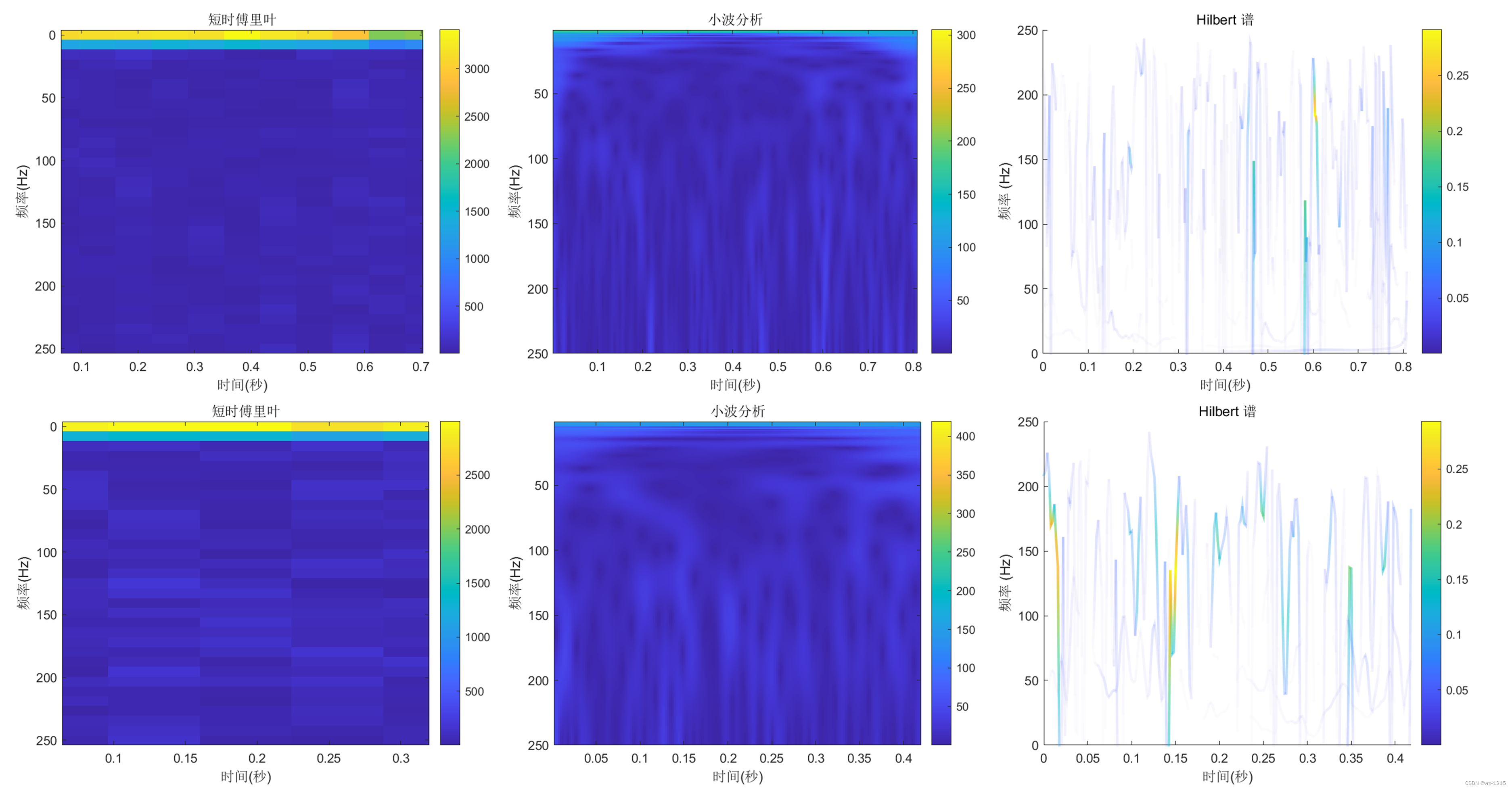
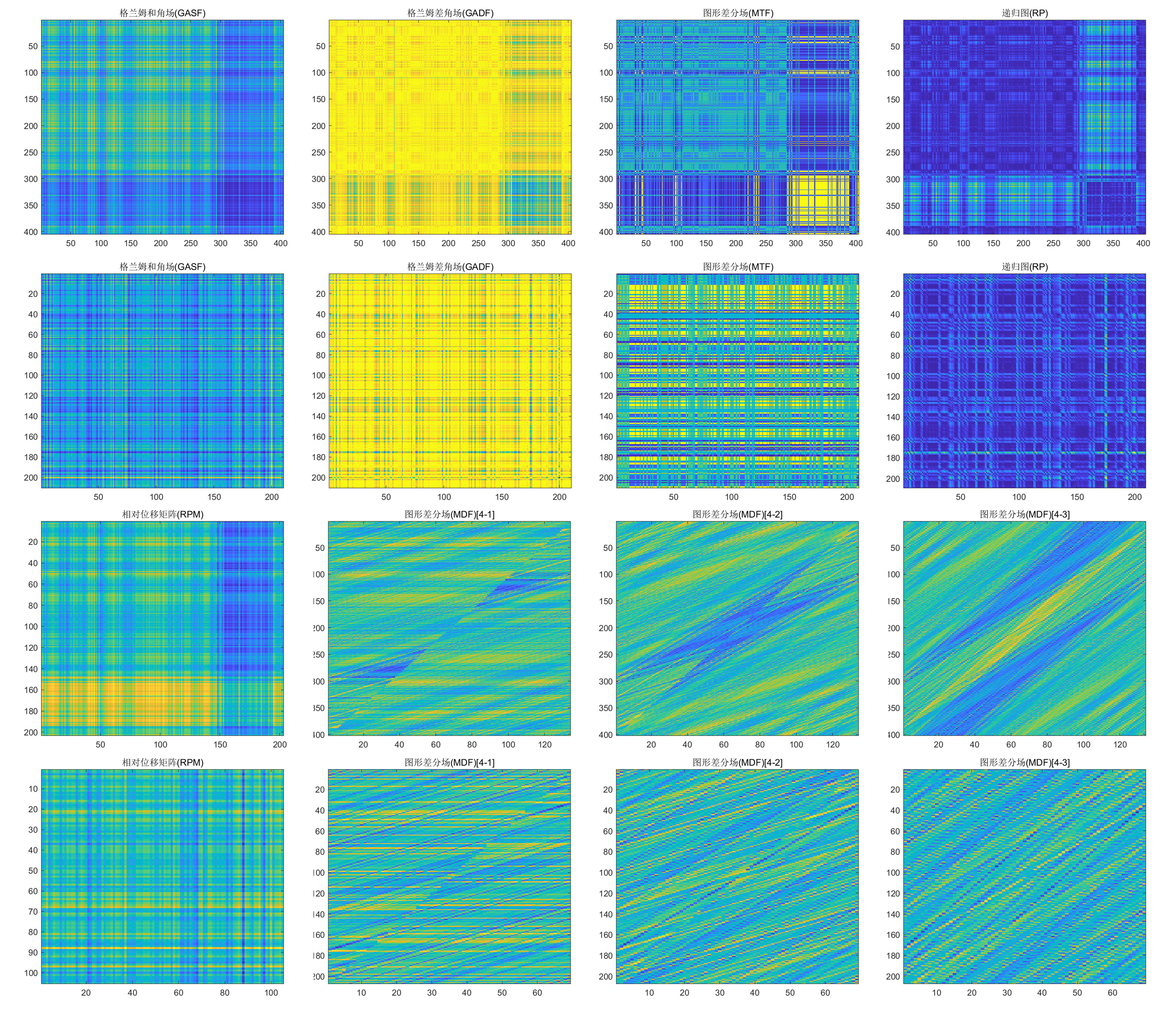
可以看出时频方法与其他方法的实验结果差别很大，时频分析方法的实验结果从图像上看没有明显的差别，这是因为时频分析方法分析的是数据的波动频率，而波动频率不是数据的异常特征；相比之下，其他的方法有明显的图像特征，会出现成块的异常特征，其中GAF、MTF、RP、RPM的实验结果相似。

部分代码为：

import pandas as pd
import matplotlib.pyplot as plt
import numpy as np
import seaborn as sns
import math

def GAF(X):
    '''
    the code of GAF
    input: the time series in raw
    output: the heatmap of GASF and GADF
    '''
    # normalization to [-1,1]
    X = ((X - np.max(X)) + (X - np.min(X))) / (np.max(X) + np.min(X))

    # generate the GASF
    gasf = X.T * X - np.sqrt(1 - np.square(X)).T * np.sqrt(1 - np.square(X))
    sns.heatmap(gasf, cbar=False, square=True, cmap='GnBu',xticklabels=False, yticklabels=False)
    # plt.show()
    plt.savefig('picture/GASF_1.jpg')

    # generate the GADF
    gadf = np.sqrt(1 - np.square(X)).T * X +  X.T * np.sqrt(1 - np.square(X))
    
    # plot the heatmap
    sns.heatmap(gadf, cbar=False, square=True, cmap='GnBu', xticklabels=False, yticklabels=False)
    # plt.show()
    plt.savefig('picture/GADF_1.jpg')

    return 0

def MTF(X):
    '''
    the code of MTF
    input: the time series in raw
    output: the heatmap of MTF
    '''
    # normalization to [0,1]
    X = (X - np.min(X)) / (np.max(X) - np.min(X))
    # the length of X
    Xlen = X.shape[1]
    # design the number of bins
    Q = 4
    # compute the temp matrix X_Q
    X_Q = np.ones([1, Xlen]) * 4
    # print(X_Q)
    temp = 0
    threshold = np.zeros([1, Q])
    for i in range(Q):
        # print((Xlen * i / Q))
        # print(np.sum(X < temp))
        while np.sum(X < temp) < (Xlen * i / Q):
            temp += 0.01
        # print(threshold.shape)
        threshold[0][i] = temp
        X_Q[np.where(X<temp)] -= 1
        # print(X_Q)
    # print(threshold)

    # generate the Markov matrix
    sum_MM = np.zeros([4,4])

    # compute the probability of Markov
    for i in range(Xlen-1):
        if X_Q[0][i] - X_Q[0][i+1] == -3:
            sum_MM[0][3] = sum_MM[0][3] + 1
        elif X_Q[0][i] - X_Q[0][i+1] == -2:
            if X_Q[0][i] == 1:
                sum_MM[0][2] = sum_MM[0][2] + 1
            elif X_Q[0][i] == 2:
                sum_MM[1][3] = sum_MM[1][3] +1
        elif X_Q[0][i] - X_Q[0][i+1] == -1:
            if X_Q[0][i] == 1:
                sum_MM[0][1] = sum_MM[0][1] + 1
            elif X_Q[0][i] == 2:
                sum_MM[1][2] = sum_MM[1][2] + 1
            elif X_Q[0][i] == 3:
                sum_MM[2][3] = sum_MM[2][3] + 1
        elif X_Q[0][i] - X_Q[0][i+1] == 0:
            if X_Q[0][i] == 1:
                sum_MM[0][0] = sum_MM[0][0] + 1
            elif X_Q[0][i] == 2:
                sum_MM[1][1] = sum_MM[1][1] + 1
            elif X_Q[0][i] == 3:
                sum_MM[2][2] = sum_MM[2][2] + 1
            elif X_Q[0][i] == 4:
                sum_MM[3][3] = sum_MM[3][3] + 1
        elif X_Q[0][i] - X_Q[0][i+1] == 1:
            if X_Q[0][i] == 2:
                sum_MM[1][0] = sum_MM[1][0] + 1
            elif X_Q[0][i] == 3:
                sum_MM[2][1] = sum_MM[2][1] + 1
            elif X_Q[0][i] == 4:
                sum_MM[3][2] = sum_MM[3][2] + 1
        elif X_Q[0][i] - X_Q[0][i+1] == 2:
            if X_Q[0][i] == 3:
                sum_MM[2][0] = sum_MM[2][0] + 1
            elif X_Q[0][i] == 4:
                sum_MM[3][1] = sum_MM[3][1] + 1
        elif X_Q[0][i] - X_Q[0][i+1] == 3:
            sum_MM[3][0] = sum_MM[3][0] + 1
    W = sum_MM
    W = W / np.sum(W,axis=1)
    # print(W)

    # generate the Markov Transform Field
    mtf = np.zeros([Xlen, Xlen])
    for i in range(Xlen):
        for j in range(Xlen):
            # print(X_Q[0][i])
            mtf[i][j] = W[int(X_Q[0][i])-1][int(X_Q[0][j])-1]
    mtf = (mtf - mtf.min()) / (mtf.max()- mtf.min()) * 4
    # generate the heatmap
    sns.heatmap(mtf,cbar=False,square=True,cmap='GnBu',xticklabels=False,yticklabels=False)
    # plt.show()
    plt.savefig('picture/MTF_1.jpg')
    return 0

def RP(X):
    # normalization to [0,1]
    X = (X - np.max(X))  / (np.max(X) + np.min(X))
    Xlen = X.shape[1]
    # convert to the phase space(第一元素是此时高度，第二个给元素为下一时刻的高度)
    S = np.zeros([Xlen-1,2])

    S[:,0] = X[0,:-1]
    S[:,1] = X[0,1:]

    # compute RRP matrix
    R = np.zeros([Xlen-1,Xlen-1])
    for i in range(Xlen-1):
        for j in range(Xlen-1):
            R[i,j] = sum(pow(S[i,:]-S[j,:],2))
    # normalization to [0,4] of RP
    R = (R - R.min()) / (R.max() - R.min()) * 4

    # show the heatmap(bwr,coolwarm,GnBu)
    sns.heatmap(R, cbar=False, square=True,cmap='GnBu',xticklabels=False,yticklabels=False)
    # plt.show()
    plt.savefig('picture/RP_1.jpg')


    return 0

def MDF(X,n):
    # normalization to [0,1]
    X = (X - np.max(X))  / (np.max(X) + np.min(X))

    # compute the length of time series and the range of d
    T = X.shape[1]
    dMax = math.floor((T-1)/(n-1))

    # initial the M,IMG
    M = np.zeros([n,T-n+1,dMax])
    
    
    # initial the dM,K
    dM = np.zeros([n-1,T-n+1,dMax])
    K = np.ones([n-1,T-n+1,dMax])   
    for d in range(dMax):
        d = d + 1
        # initial the s
        s = np.zeros([T-(n-1)*d])
        for i in range(T-(n-1)*d):
            s[i] = i
        for ImageIndex in range(n):
            # print(s+ImageIndex*d)
            s_index = (s+ImageIndex*d).astype(np.int16)
            s = s.astype(np.int16)
            # print(X[0,s_index])
            M[ImageIndex,s,d-1] = X[0,s_index]

            
            if ImageIndex >= 1:
                # motif difference
                dM[ImageIndex-1,s,d-1] = M[ImageIndex,s,d-1] - M[ImageIndex-1,s,d-1]
                # K
                K[ImageIndex-1,s,d-1] = np.zeros([T-(n-1)*d])
    
    IMG = np.zeros([n-1,T-n+1,dMax])
    for ImageIndex in range(n-1):
        # G
        G = dM[ImageIndex]
        # the rot180 of G
        G_1 = G.reshape(1,(T-n+1)*dMax)
        G_2 = G_1[0][::-1]
        G_rot = G_2.reshape(T-n+1,dMax)
        IMG[ImageIndex,:,:] = G + K[ImageIndex] * G_rot
        sns.heatmap(IMG[ImageIndex,:,:].T, cbar=False, square=True, cmap='GnBu', xticklabels=False, yticklabels=False)
        # plt.show()
        # print(IMG)
        plt.savefig('picture/MDF'+'%d'%ImageIndex+'_1.jpg')
    return 0

if __name__ == "__main__":

    # get the data
    data = pd.read_csv(filename)

    # dataframe to numpy
    data_numpy = data.values

    # show the motif of the data
    fig1 = plt.figure(1)
    plt.plot(range(len(data_numpy)), data_numpy)
    plt.xlim([0, len(data_numpy)-1])
    plt.ylim([20, 120])
    plt.ylabel('speed')
    plt.xlabel('time index')
    plt.title('time series of normal')
    # plt.show()
    plt.savefig('picture/normal.jpg')

    # GAF(data_numpy.T)

    # MTF(data_numpy.T)

    # RP(data_numpy.T)

    n = 4
    MDF(data_numpy.T,n)

    # x=list()
    # temp = list()
    # for t in np.arange(0,10,0.01):
    #     temp.append(t)
    #     x.append(math.sin(t))
    # print(x)
    # plt.plot(temp,x)
    # plt.show()

5 总结与分析

本文详细介绍了目前时间序列转二维图像的方法及其应用现状；同时以交通异常检测场景为例，对各个方法做了案例分析。各项研究结果表明，将时间序列数据转化为二维图像，利用成熟的计算机视觉技术进行特征提取和识别，可以有效提高效果，这将有助于时间序列数据的研究。总的来说，此类方法之所以更优于传统的时间序列分析方法，主要是因为有以下几点：

1. 转化的过程本质上是一种升维的过程，这意味着信息量增加，比如增加了不同时刻数据值之间的关系表征；
2. 转化的过程同时也是一种数据处理过程，凸显了数据的主要特征；
3. 可以借助计算机视觉领域中的特征提取机制进行高效地特征提取；

如今，随着数据采集技术的不断提升和数据采集设备的广泛铺设，众多场景下的时间序列数据呈大体量涌现，急需高效的数据分析方法。而将时间序列转化为二维图像，借助现有的图像领域的研究成果进行分析，是一个新的突破途径。该领域还有一些待挖掘的研究点，比如转化过程中的数据不丢失问题。目前，时间序列分析领域相对于图像领域，在研究进展上还未有较大的突破，希望本文可以提供给相关领域的研究者一个新的视角。

【若觉文章质量良好且有用，请别忘了点赞收藏加关注，这将是我继续分享的动力，万分感谢！】

6 参考文献

---

[1] Fu T. A review on time series data mining[J]. Engineering Applications of Artificial Intelligence, 2011, 24(1): 164-181.

[2] Fawaz H I, Forestier G, Weber J, et al. Deep learning for time series classification: a review[J]. Data mining and knowledge discovery, 2019, 33(4): 917-963.

[3] LeCun Y, Bottou L, Bengio Y, et al. Gradient-based learning applied to document recognition[J]. Proceedings of the IEEE, 1998, 86(11): 2278-2324.

[4] Krizhevsky A, Sutskever I, Hinton G E. Imagenet classification with deep convolutional neural networks[J]. Advances in neural information processing systems, 2012, 25: 1097-1105.

[5] He K, Zhang X, Ren S, et al. Deep residual learning for image recognition[C]//Proceedings of the IEEE conference on computer vision and pattern recognition. 2016: 770-778.

[6] Tan M, Le Q. Efficientnet: Rethinking model scaling for convolutional neural networks[C]//International Conference on Machine Learning. PMLR, 2019: 6105-6114.

[7] Gabor D. Theory of communication. Part 1: The analysis of information[J]. Journal of the Institution of Electrical Engineers-Part III: Radio and Communication Engineering, 1946, 93(26): 429-441.

[8] Morlet J, Arens G, Fourgeau E, et al. Wave propagation and sampling theory—Part II: Sampling theory and complex waves[J]. Geophysics, 1982, 47(2): 222-236.

[9] Huang N E, Shen Z, Long S R, et al. The empirical mode decomposition and the Hilbert spectrum for nonlinear and non-stationary time series analysis[J]. Proceedings of the Royal Society of London. Series A: mathematical, physical and engineering sciences, 1998, 454(1971): 903-995.

[10] Wang Z, Oates T. Imaging time-series to improve classification and imputation[C]//Twenty-Fourth International Joint Conference on Artificial Intelligence. 2015.

[11] Hatami N, Gavet Y, Debayle J. Classification of time-series images using deep convolutional neural networks[C]//Tenth international conference on machine vision (ICMV 2017). International Society for Optics and Photonics, 2018, 10696: 106960Y.

[12] Zhang Y, Chen X. Motif Difference Field: A Simple and Effective Image Representation of Time Series for Classification[J]. arXiv preprint arXiv:2001.07582, 2020.

[13] Chen W, Shi K. A deep learning framework for time series classification using Relative Position Matrix and Convolutional Neural Network[J]. Neurocomputing, 2019, 359: 384-394.

[14] Eckmann J P, Kamphorst S O, Ruelle D. Recurrence plots of dynamical systems[J]. World Scientific Series on Nonlinear Science Series A, 1995, 16: 441-446.

[15] Davis C. The norm of the Schur product operation[J]. Numerische Mathematik, 1962, 4(1): 343-344.

[16] Liu X, Cai H, Zhong R, et al. Learning traffic as images for incident detection using convolutional neural networks[J]. IEEE Access, 2020, 8: 7916-7924.

[17] Fahim S R, Sarker Y, Sarker S K, et al. Self attention convolutional neural network with time series imaging based feature extraction for transmission line fault detection and classification[J]. Electric Power Systems Research, 2020, 187: 106437.

[18] Qin Z, Zhang Y, Meng S, et al. Imaging and fusing time series for wearable sensor-based human activity recognition[J]. Information Fusion, 2020, 53: 80-87.

[19] Fahim S R, Sarker Y, Sarker S K, et al. Self attention convolutional neural network with time series imaging based feature extraction for transmission line fault detection and classification[J]. Electric Power Systems Research, 2020, 187: 106437.

[20] Kiangala K S, Wang Z. An effective predictive maintenance framework for conveyor motors using dual time-series imaging and convolutional neural network in an industry 4.0 environment[J]. Ieee Access, 2020, 8: 121033-121049.

[21] 骆俊锦, 王万良, 王铮, 等. 基于时序二维化和卷积特征融合的表面肌电信号分类方法[J]. 模式识别与人工智能, 2020, 33(7): 588-599.

[22] Barra S, Carta S M, Corriga A, et al. Deep learning and time series-to-image encoding for financial forecasting[J]. IEEE/CAA Journal of Automatica Sinica, 2020, 7(3): 683-692.

[23] Fahim M, Fraz K, Sillitti A. TSI: Time series to imaging based model for detecting anomalous energy consumption in smart buildings[J]. Information Sciences, 2020, 523: 1-13.

[24] Li X, Kang Y, Li F. Forecasting with time series imaging[J]. Expert Systems with Applications, 2020, 160: 113680.

[25] Hsueh Y, Ittangihala V R, Wu W B, et al. Condition monitor system for rotation machine by CNN with recurrence plot[J]. Energies, 2019, 12(17): 3221.

[26] Zhang Y, Gan F, Chen X. Motif Difference Field: An Effective Image-based Time Series Classification and Applications in Machine Malfunction Detection[C]//2020 IEEE 4th Conference on Energy Internet and Energy System Integration (EI2). IEEE, 3079-3083.

---