import cv2
 import numpy as np
 from matplotlib import pyplot as plt
 img = cv2.imread('sample.png',0) # Using 0 to read image in grayscale mode
 plt.imshow(img, cmap='gray')  #cmap is used to specify imshow that the image is in greyscale
 plt.xticks([]), plt.yticks([])  # remove tick marks
 plt.show()
f = np.fft.fft2(img) #the image 'img' is passed to np.fft.fft2() to compute its 2D Discrete Fourier transform f
mag = 20*np.log(np.abs(f))
plt.imshow(mag, cmap = 'gray') #cmap='gray' parameter to indicate that the image should be displayed in grayscale.
plt.title('Magnitude Spectrum')
plt.xticks([]), plt.yticks([])
plt.show()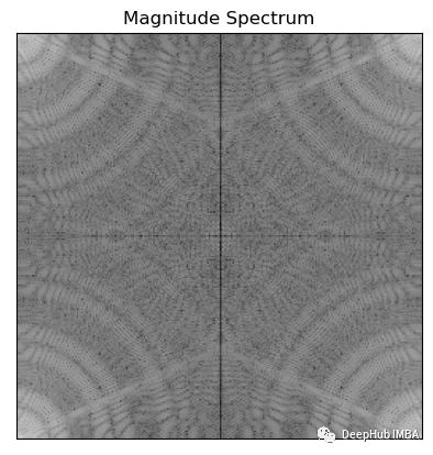 上面代码使用np.abs()计算傅里叶变换f的幅度,np.log()转换为对数刻度,然后乘以20得到以分贝为单位的幅度。这样做是为了使幅度谱更容易可视化和解释。
fshift = np.fft.fftshift(f)
 mag = 20*np.log(np.abs(fshift))
 plt.imshow(mag, cmap = 'gray')
 plt.title('Centered Spectrum'), plt.xticks([]), plt.yticks([])
 plt.show()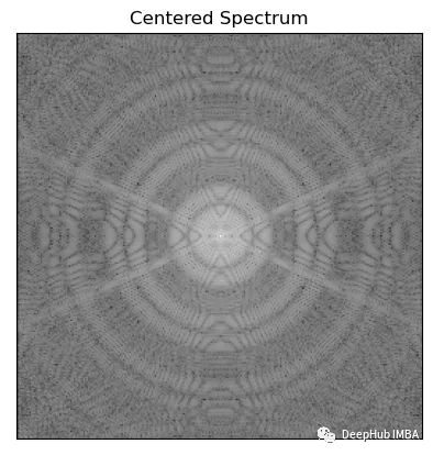
import math
 def distance(point1,point2):
     return math.sqrt((point1[0]-point2[0])**2 + (point1[1]-point2[1])**2)

 def idealFilterLP(D0,imgShape):
     base = np.zeros(imgShape[:2])
     rows, cols = imgShape[:2]
     center = (rows/2,cols/2)
     for x in range(cols):
         for y in range(rows):
             if distance((y,x),center) < D0:
                 base[y,x] = 1
     return base

 def idealFilterHP(D0,imgShape):
     base = np.ones(imgShape[:2])
     rows, cols = imgShape[:2]
     center = (rows/2,cols/2)
     for x in range(cols):
         for y in range(rows):
             if distance((y,x),center) < D0:
                 base[y,x] = 0
return baseimport math
def distance(point1,point2):
return math.sqrt((point1[0]-point2[0])**2 + (point1[1]-point2[1])**2)
def gaussianLP(D0,imgShape):
base = np.zeros(imgShape[:2])
rows, cols = imgShape[:2]
center = (rows/2,cols/2)
for x in range(cols):
for y in range(rows):
base[y,x] = math.exp(((-distance((y,x),center)**2)/(2*(D0**2))))
return base
def gaussianHP(D0,imgShape):
base = np.zeros(imgShape[:2])
rows, cols = imgShape[:2]
center = (rows/2,cols/2)
for x in range(cols):
for y in range(rows):
base[y,x] = 1 - math.exp(((-distance((y,x),center)**2)/(2*(D0**2))))
return basefig, ax = plt.subplots(2, 2) # create a 2x2 grid of subplots
fig.suptitle('Filters') # set the title for the entire figure
# plot the first image in the top-left subplot
im1 = ax[0, 0].imshow(np.abs(idealFilterLP(50, img.shape)), cmap='gray')
ax[0, 0].set_title('Low Pass Filter of Diameter 50 px')
ax[0, 0].set_xticks([])
ax[0, 0].set_yticks([])
# plot the second image in the top-right subplot
im2 = ax[0, 1].imshow(np.abs(idealFilterHP(50, img.shape)), cmap='gray')
ax[0, 1].set_title('High Pass Filter of Diameter 50 px')
ax[0, 1].set_xticks([])
ax[0, 1].set_yticks([])
# plot the third image in the bottom-left subplot
im3 = ax[1, 0].imshow(np.abs(gaussianLP(50 ,img.shape)), cmap='gray')
ax[1, 0].set_title('Gaussian Filter of Diameter 50 px')
ax[1, 0].set_xticks([])
ax[1, 0].set_yticks([])
# plot the fourth image in the bottom-right subplot
im4 = ax[1, 1].imshow(np.abs(gaussianHP(50 ,img.shape)), cmap='gray')
ax[1, 1].set_title('Gaussian Filter of Diameter 50 px')
ax[1, 1].set_xticks([])
ax[1, 1].set_yticks([])
# adjust the spacing between subplots
fig.subplots_adjust(wspace=0.5, hspace=0.5)
# save the figure to a file
fig.savefig('filters.png', bbox_inches='tight')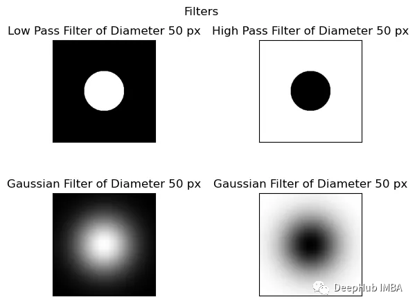 相乘过滤器和移位的图像得到过滤图像为了获得具有所需频率响应的最终滤波图像,关键是在频域中对移位后的图像与滤波器进行逐点乘法。这个过程将两个图像元素的对应像素相乘。例如,当应用低通滤波器时,我们将对移位的傅里叶变换图像与低通滤波器逐点相乘。此操作抑制高频并保留低频,对于高通滤波器反之亦然。这个乘法过程对于去除不需要的频率和增强所需的频率是必不可少的,从而产生更清晰和更清晰的图像。它使我们能够获得期望的频率响应,并在频域获得最终滤波图像。
fig, ax = plt.subplots()
im = ax.imshow(np.log(1+np.abs(fftshifted_image * idealFilterLP(50,img.shape))), cmap='gray')
ax.set_title('Filtered Image in Frequency Domain')
ax.set_xticks([])
ax.set_yticks([])
fig.savefig('filtered image in freq domain.png', bbox_inches='tight')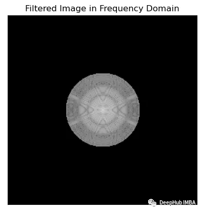 在可视化傅里叶频谱时,使用np.log(1+np.abs(x))和20*np.log(np.abs(x))之间的选择是个人喜好的问题,可以取决于具体的应用程序。一般情况下会使用Np.log (1+np.abs(x)),因为它通过压缩数据的动态范围来帮助更清晰地可视化频谱。这是通过取数据绝对值的对数来实现的,并加上1以避免取零的对数。而20*np.log(np.abs(x))将数据按20倍缩放,并对数据的绝对值取对数,这可以更容易地看到不同频率之间较小的幅度差异。但是它不会像np.log(1+np.abs(x))那样压缩数据的动态范围。这两种方法都有各自的优点和缺点,最终取决于具体的应用程序和个人偏好。
fig, ax = plt.subplots()
 im = ax.imshow(np.log(1+np.abs(np.fft.ifftshift(fftshifted_image * idealFilterLP(50,img.shape)))), cmap='gray')
 ax.set_title('Filtered Image inverse fft shifted')
 ax.set_xticks([])
 ax.set_yticks([])

 fig.savefig('filtered image inverse fft shifted.png', bbox_inches='tight')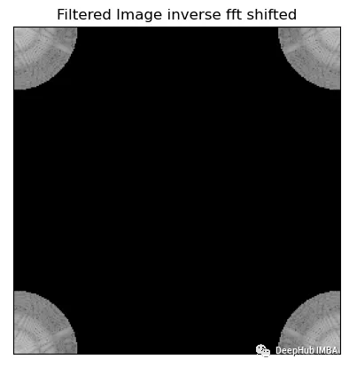
fig, ax = plt.subplots()
 im = ax.imshow(np.log(1+np.abs(np.fft.ifft2(np.fft.ifftshift(fftshifted_image * idealFilterLP(50,img.shape))))), cmap='gray')
 ax.set_title('Final Filtered Image In Spatial Domain')
 ax.set_xticks([])
 ax.set_yticks([])

 fig.savefig('final filtered image.png', bbox_inches='tight')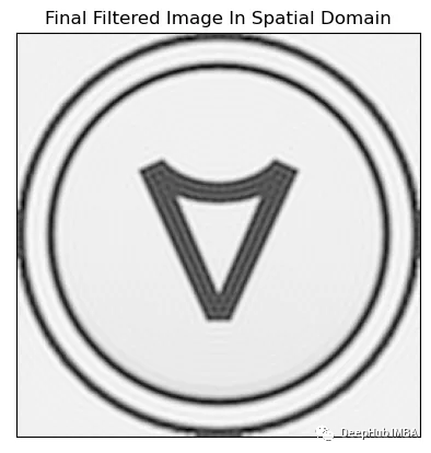
def Freq_Trans(image, filter_used):
     img_in_freq_domain = np.fft.fft2(image)

     # Shift the zero-frequency component to the center of the frequency spectrum
     centered = np.fft.fftshift(img_in_freq_domain)

     # Multiply the filter with the centered spectrum
     filtered_image_in_freq_domain = centered * filter_used

     # Shift the zero-frequency component back to the top-left corner of the frequency spectrum
     inverse_fftshift_on_filtered_image = np.fft.ifftshift(filtered_image_in_freq_domain)

     # Apply the inverse Fourier transform to obtain the final filtered image
     final_filtered_image = np.fft.ifft2(inverse_fftshift_on_filtered_image)

return img_in_freq_domain,centered,filter_used,filtered_image_in_freq_domain,inverse_fftshift_on_filtered_image,final_filtered_imagefig, axs = plt.subplots(12, 7, figsize=(30, 60))
filters = [(f, d) for f in [idealFilterLP, idealFilterHP, gaussianLP, gaussianHP] for d in [50, 100, 150]]
for row, (filter_name, filter_diameter) in enumerate(filters):
# Plot each filter output on a separate subplot
result = Freq_Trans(img, filter_name(filter_diameter, img.shape))
for col, title, img_array in zip(range(7),
["Original Image", "Spectrum", "Centered Spectrum", f"{filter_name.__name__} of Diameter {filter_diameter} px",
f"Centered Spectrum multiplied by {filter_name.__name__}", "Decentralize", "Processed Image"],
[img, np.log(1+np.abs(result[0])), np.log(1+np.abs(result[1])), np.abs(result[2]), np.log(1+np.abs(result[3])),
np.log(1+np.abs(result[4])), np.abs(result[5])]):
axs[row, col].imshow(img_array, cmap='gray')
axs[row, col].set_title(title)
plt.tight_layout()
plt.savefig('all_processess.png', bbox_inches='tight')
plt.show()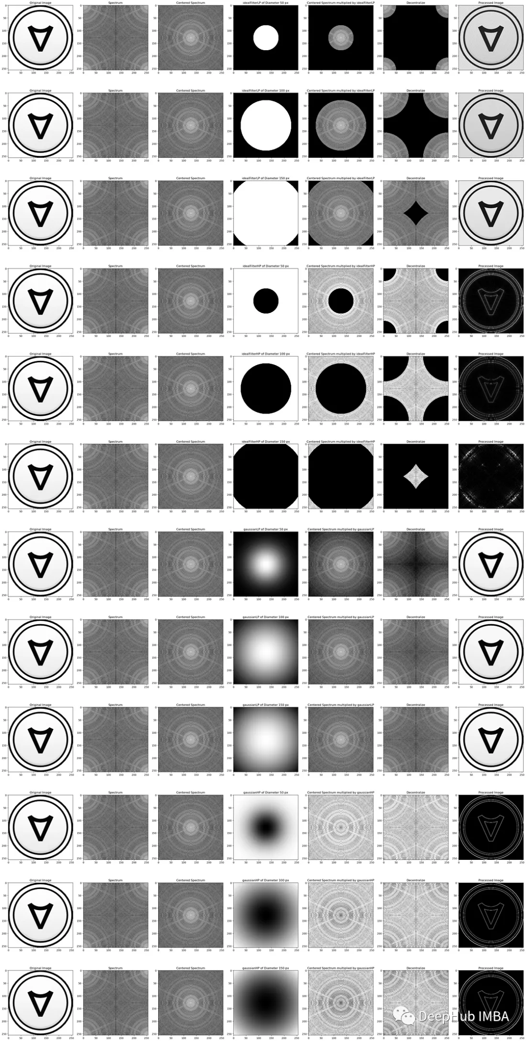 可以看到,当改变圆形掩膜的直径时,对图像清晰度的影响会有所不同。随着直径的增加,更多的频率被抑制,从而产生更平滑的图像和更少的细节。减小直径允许更多的频率通过,从而产生更清晰的图像和更多的细节。为了达到理想的效果,选择合适的直径是很重要的,因为使用太小的直径会导致过滤器不够有效,而使用太大的直径会导致丢失太多的细节。一般来说,高斯滤波器由于其平滑性和鲁棒性,更常用于图像处理任务。在某些应用中,需要更尖锐的截止,理想滤波器可能更适合。利用FFT修改图像频率是一种有效的降低噪声和提高图像锐度的方法。这包括使用FFT将图像转换到频域,使用适当的技术过滤噪声,并使用反FFT将修改后的图像转换回空间域。通过理解和实现这些技术,我们可以提高各种应用程序的图像质量。
 关闭。这个问题是opinion-based.它目前不接受答案。想要改进这个问题?更新问题,以便editingthispost可以用事实和引用来回答它.关闭4年前。Improvethisquestion我想在固定时间创建一系列低音和高音调的哔哔声。例如:在150毫秒时发出高音调的蜂鸣声在151毫秒时发出低音调的蜂鸣声200毫秒时发出低音调的蜂鸣声250毫秒的高音调蜂鸣声有没有办法在Ruby或Python中做到这一点?我真的不在乎输出编码是什么(.wav、.mp3、.ogg等等),但我确实想创建一个输出文件。
Rackup通过Rack的默认处理程序成功运行任何Rack应用程序。例如:classRackAppdefcall(environment)['200',{'Content-Type'=>'text/html'},["Helloworld"]]endendrunRackApp.new但是当最后一行更改为使用Rack的内置CGI处理程序时,rackup给出“NoMethodErrorat/undefinedmethod`call'fornil:NilClass”:Rack::Handler::CGI.runRackApp.newRack的其他内置处理程序也提出了同样的反对意见。例如Rack
我有带有Logo图像的公司模型has_attached_file:logo我用他们的Logo创建了许多公司。现在,我需要添加新样式has_attached_file:logo,:styles=>{:small=>"30x15>",:medium=>"155x85>"}我是否应该重新上传所有旧数据以重新生成新样式?我不这么认为……或者有什么rake任务可以重新生成样式吗? 最佳答案 参见Thumbnail-Generation.如果rake任务不适合你,你应该能够在控制台中使用一个片段来调用重新处理!关于相关公司
这个问题在这里已经有了答案:关闭10年前。PossibleDuplicate:Pythonconditionalassignmentoperator对于这样一个简单的问题表示歉意,但是谷歌搜索||=并不是很有帮助;)Python中是否有与Ruby和Perl中的||=语句等效的语句?例如:foo="hey"foo||="what"#assignfooifit'sundefined#fooisstill"hey"bar||="yeah"#baris"yeah"另外,类似这样的东西的通用术语是什么?条件分配是我的第一个猜测,但Wikipediapage跟我想的不太一样。
什么是ruby的rack或python的Java的wsgi?还有一个路由库。 最佳答案 来自Python标准PEP333:Bycontrast,althoughJavahasjustasmanywebapplicationframeworksavailable,Java's"servlet"APImakesitpossibleforapplicationswrittenwithanyJavawebapplicationframeworktoruninanywebserverthatsupportstheservletAPI.ht
华为OD机试题本篇题目:明明的随机数题目输入描述输出描述:示例1输入输出说明代码编写思路最近更新的博客华为od2023|什么是华为od,od薪资待遇,od机试题清单华为OD机试真题大全,用Python解华为机试题|机试宝典【华为OD机试】全流程解析+经验分享,题型分享,防作弊指南华为o
我想解析一个已经存在的.mid文件,改变它的乐器,例如从“acousticgrandpiano”到“violin”,然后将它保存回去或作为另一个.mid文件。根据我在文档中看到的内容,该乐器通过program_change或patch_change指令进行了更改,但我找不到任何在已经存在的MIDI文件中执行此操作的库.他们似乎都只支持从头开始创建的MIDI文件。 最佳答案 MIDIpackage会为您完成此操作,但具体方法取决于midi文件的原始内容。一个MIDI文件由一个或多个音轨组成,每个音轨是十六个channel中任何一个上的
本文主要介绍在使用Selenium进行自动化测试或者任务时,对于使用了iframe的页面,如何定位iframe中的元素文章目录场景描述解决方案具体代码场景描述当我们在使用Selenium进行自动化测试的时候,可能会遇到一些界面或者窗体是使用HTML的iframe标签进行承载的。对于iframe中的标签,如果直接查找是无法找到的,会抛出没有找到元素的异常。比如近在咫尺的例子就是,CSDN的登录窗体就是使用的iframe,大家可以尝试通过F12开发者模式查看到的tag_name,class_name,id或者xpath来定位中的页面元素,会抛出NoSuchElementException异常。解决
目录前言滤波电路科普主要分类实际情况单位的概念常用评价参数函数型滤波器简单分析滤波电路构成低通滤波器RC低通滤波器RL低通滤波器高通滤波器RC高通滤波器RL高通滤波器部分摘自《LC滤波器设计与制作》,侵权删。前言最近需要学习放大电路和滤波电路,但是由于只在之前做音乐频谱分析仪的时候简单了解过一点点运放,所以也是相当从零开始学习了。滤波电路科普主要分类滤波器:主要是从不同频率的成分中提取出特定频率的信号。有源滤波器:由RC元件与运算放大器组成的滤波器。可滤除某一次或多次谐波,最普通易于采用的无源滤波器结构是将电感与电容串联,可对主要次谐波(3、5、7)构成低阻抗旁路。无源滤波器:无源滤波器,又称
我正在尝试使用Ruby2.0.0和Rails4.0.0提供的API从imgur中提取图像。我已尝试按照Ruby2.0.0文档中列出的各种方式构建http请求,但均无济于事。代码如下:require'net/http'require'net/https'defimgurheaders={"Authorization"=>"Client-ID"+my_client_id}path="/3/gallery/image/#{img_id}.json"uri=URI("https://api.imgur.com"+path)request,data=Net::HTTP::Get.new(path