本文参考【中文】【吴恩达课后编程作业】Course 2 - 改善深层神经网络 - 第一周作业(1&2&3)_何宽的博客-CSDN博客,加上自己的理解,方便自己以后的学习。我觉得这次理解起来还是蛮简单的,就是知识点比较多
让我们跟着这篇博客对比着来学习吧!
本文所使用的资料已上传到百度网盘【点击下载】,提取码:imgq ,请在开始之前下载好所需资料,或者在本文底部copy资料代码。
我们在开始之前说一下我们要干什么。在这篇文章中,我们要干三件事:
1. 初始化参数:
	1.1:使用0来初始化参数。
	1.2:使用随机数来初始化参数。
	1.3:使用抑梯度异常初始化参数(参见视频中的梯度消失和梯度爆炸)。
2. 正则化模型:
	2.1:使用二范数对二分类模型正则化,尝试避免过拟合。
	2.2:使用随机删除节点的方法精简模型,同样是为了尝试避免过拟合。
3. 梯度校验  :对模型使用梯度校验,检测它是否在梯度下降的过程中出现误差过大的情况。
我们就开始导入相关的库:
import numpy as np
import matplotlib.pyplot as plt
import sklearn
import sklearn.datasets
import init_utils   #第一部分,初始化
import reg_utils    #第二部分,正则化
import gc_utils     #第三部分,梯度校验
import testCase     #第四部分,梯度检查
plt.rcParams['figure.figsize'] = (7.0, 4.0) # set default size of plots
plt.rcParams['image.interpolation'] = 'nearest'
plt.rcParams['image.cmap'] = 'gray'我们在初始化之前,我们来看看我们的数据集是怎样的:
train_X, train_Y, test_X, test_Y = init_utils.load_dataset(is_plot=True)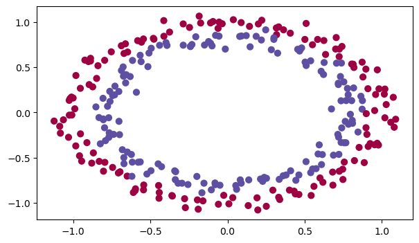
我们将要建立一个分类器把蓝点和红点分开,在之前我们已经实现过一个3层的神经网络,我们将对它进行初始化:
我们将会尝试下面三种初始化方法:
parameters['W' + str(l)] = np.zeros((layers_dims[l], layers_dims[l - 1]))parameters['W' + str(l)] = np.random.randn(layers_dims[l], layers_dims[l - 1]) * 10parameters['W' + str(l)] = np.random.randn(layers_dims[l], layers_dims[l - 1]) * np.sqrt(2 / layers_dims[l - 1])首先我们来看看我们的模型是怎样的:
def model(X,Y,learning_rate=0.01,num_iterations=15000,print_cost=True,initialization="he",is_polt=True):
    """
    实现一个三层的神经网络:LINEAR ->RELU -> LINEAR -> RELU -> LINEAR -> SIGMOID

    参数:
        X - 输入的数据,维度为(2, 要训练/测试的数量)
        Y - 标签,【0 | 1】,维度为(1,对应的是输入的数据的标签)
        learning_rate - 学习速率
        num_iterations - 迭代的次数
        print_cost - 是否打印成本值,每迭代1000次打印一次
        initialization - 字符串类型,初始化的类型【"zeros" | "random" | "he"】
        is_polt - 是否绘制梯度下降的曲线图
    返回
        parameters - 学习后的参数
    """
    grads = {}
    costs = []
    m = X.shape[1]
    layers_dims = [X.shape[0],10,5,1]

    #选择初始化参数的类型
    if initialization == "zeros":
        parameters = initialize_parameters_zeros(layers_dims)
    elif initialization == "random":
        parameters = initialize_parameters_random(layers_dims)
    elif initialization == "he":
        parameters = initialize_parameters_he(layers_dims)
    else :
        print("错误的初始化参数!程序退出")

    #开始学习
    for i in range(0,num_iterations):
        #前向传播
        a3 , cache = init_utils.forward_propagation(X,parameters)

        #计算成本
        cost = init_utils.compute_loss(a3,Y)

        #反向传播
        grads = init_utils.backward_propagation(X,Y,cache)

        #更新参数
        parameters = init_utils.update_parameters(parameters,grads,learning_rate)

        #记录成本
        if i % 1000 == 0:
            costs.append(cost)
            #打印成本
            if print_cost:
                print("第" + str(i) + "次迭代,成本值为:" + str(cost))


    #学习完毕,绘制成本曲线
    if is_polt:
        plt.plot(costs)
        plt.ylabel('cost')
        plt.xlabel('iterations (per hundreds)')
        plt.title("Learning rate =" + str(learning_rate))
        plt.show()

    #返回学习完毕后的参数
    return parameters
模型我们可以简单地看一下,我们这就开始尝试一下这三种初始化。
def initialize_parameters_zeros(layers_dims):
    """
    将模型的参数全部设置为0

    参数:
        layers_dims - 列表,模型的层数和对应每一层的节点的数量
    返回
        parameters - 包含了所有W和b的字典
            W1 - 权重矩阵,维度为(layers_dims[1], layers_dims[0])
            b1 - 偏置向量,维度为(layers_dims[1],1)
            ···
            WL - 权重矩阵,维度为(layers_dims[L], layers_dims[L -1])
            bL - 偏置向量,维度为(layers_dims[L],1)
    """
    parameters = {}

    L = len(layers_dims) #网络层数

    for l in range(1,L):
        parameters["W" + str(l)] = np.zeros((layers_dims[l],layers_dims[l-1]))
        parameters["b" + str(l)] = np.zeros((layers_dims[l],1))

        #使用断言确保我的数据格式是正确的
        assert(parameters["W" + str(l)].shape == (layers_dims[l],layers_dims[l-1]))
        assert(parameters["b" + str(l)].shape == (layers_dims[l],1))

    return parameters
我们这就来测试一下:
parameters = initialize_parameters_zeros([3,2,1])
print("W1 = " + str(parameters["W1"]))
print("b1 = " + str(parameters["b1"]))
print("W2 = " + str(parameters["W2"]))
print("b2 = " + str(parameters["b2"]))
W1 = [[0. 0. 0.] [0. 0. 0.]] b1 = [[0.] [0.]] W2 = [[0. 0.]] b2 = [[0.]]
我们可以看到W和b全部被初始化为0了,那么我们使用这些参数来训练模型,结果会怎样呢?
parameters = model(train_X, train_Y, initialization = "zeros",is_polt=True)第0次迭代,成本值为:0.6931471805599453 第1000次迭代,成本值为:0.6931471805599453 第2000次迭代,成本值为:0.6931471805599453 第3000次迭代,成本值为:0.6931471805599453 第4000次迭代,成本值为:0.6931471805599453 第5000次迭代,成本值为:0.6931471805599453 第6000次迭代,成本值为:0.6931471805599453 第7000次迭代,成本值为:0.6931471805599453 第8000次迭代,成本值为:0.6931471805599453 第9000次迭代,成本值为:0.6931471805599453 第10000次迭代,成本值为:0.6931471805599455 第11000次迭代,成本值为:0.6931471805599453 第12000次迭代,成本值为:0.6931471805599453 第13000次迭代,成本值为:0.6931471805599453 第14000次迭代,成本值为:0.6931471805599453
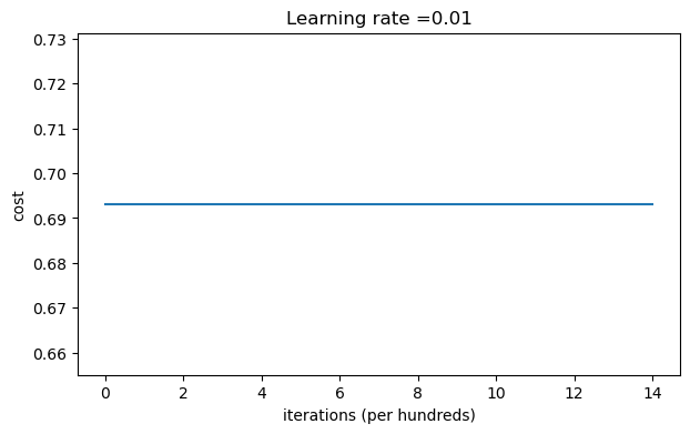
从上图中我们可以看到学习率一直没有变化,也就是说这个模型根本没有学习。我们来看看预测的结果怎么样:
print ("训练集:")
predictions_train = init_utils.predict(train_X, train_Y, parameters)
print ("测试集:")
predictions_test = init_utils.predict(test_X, test_Y, parameters)
训练集: Accuracy: 0.5 测试集: Accuracy: 0.5
性能确实很差,而且成本并没有真正降低,算法的性能也比随机猜测要好。为什么?让我们看看预测和决策边界的细节:
print("predictions_train = " + str(predictions_train))
print("predictions_test = " + str(predictions_test))

plt.title("Model with Zeros initialization")
axes = plt.gca()
axes.set_xlim([-1.5, 1.5])
axes.set_ylim([-1.5, 1.5])
init_utils.plot_decision_boundary(lambda x: init_utils.predict_dec(parameters, x.T), train_X, train_Y)
predictions_train = [[0 0 0 0 0 0 0 0 0 0 0 0 0 0 0 0 0 0 0 0 0 0 0 0 0 0 0 0 0 0 0 0 0 0 0 0 0 0 0 0 0 0 0 0 0 0 0 0 0 0 0 0 0 0 0 0 0 0 0 0 0 0 0 0 0 0 0 0 0 0 0 0 0 0 0 0 0 0 0 0 0 0 0 0 0 0 0 0 0 0 0 0 0 0 0 0 0 0 0 0 0 0 0 0 0 0 0 0 0 0 0 0 0 0 0 0 0 0 0 0 0 0 0 0 0 0 0 0 0 0 0 0 0 0 0 0 0 0 0 0 0 0 0 0 0 0 0 0 0 0 0 0 0 0 0 0 0 0 0 0 0 0 0 0 0 0 0 0 0 0 0 0 0 0 0 0 0 0 0 0 0 0 0 0 0 0 0 0 0 0 0 0 0 0 0 0 0 0 0 0 0 0 0 0 0 0 0 0 0 0 0 0 0 0 0 0 0 0 0 0 0 0 0 0 0 0 0 0 0 0 0 0 0 0 0 0 0 0 0 0 0 0 0 0 0 0 0 0 0 0 0 0 0 0 0 0 0 0 0 0 0 0 0 0 0 0 0 0 0 0 0 0 0 0 0 0 0 0 0 0 0 0 0 0 0 0 0 0 0 0 0 0 0 0 0 0 0 0 0 0]] predictions_test = [[0 0 0 0 0 0 0 0 0 0 0 0 0 0 0 0 0 0 0 0 0 0 0 0 0 0 0 0 0 0 0 0 0 0 0 0 0 0 0 0 0 0 0 0 0 0 0 0 0 0 0 0 0 0 0 0 0 0 0 0 0 0 0 0 0 0 0 0 0 0 0 0 0 0 0 0 0 0 0 0 0 0 0 0 0 0 0 0 0 0 0 0 0 0 0 0 0 0 0 0]]
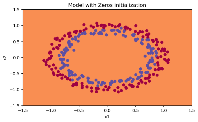
分类失败。
为了打破对称性,我们可以随机地把参数赋值。在随机初始化之后,每个神经元可以开始学习其输入的不同功能,我们还会设置比较大的参数值,看看会发生什么。
def initialize_parameters_random(layers_dims):
    """
    参数:
        layers_dims - 列表,模型的层数和对应每一层的节点的数量
    返回
        parameters - 包含了所有W和b的字典
            W1 - 权重矩阵,维度为(layers_dims[1], layers_dims[0])
            b1 - 偏置向量,维度为(layers_dims[1],1)
            ···
            WL - 权重矩阵,维度为(layers_dims[L], layers_dims[L -1])
            b1 - 偏置向量,维度为(layers_dims[L],1)
    """

    np.random.seed(3)               # 指定随机种子
    parameters = {}
    L = len(layers_dims)            # 层数

    for l in range(1, L):
        parameters['W' + str(l)] = np.random.randn(layers_dims[l], layers_dims[l - 1])*10 #使用10倍缩放
        parameters['b' + str(l)] = np.zeros((layers_dims[l], 1))

        #使用断言确保我的数据格式是正确的
        assert(parameters["W" + str(l)].shape == (layers_dims[l],layers_dims[l-1]))
        assert(parameters["b" + str(l)].shape == (layers_dims[l],1))

    return parameters
我们可以来测试一下:
parameters = initialize_parameters_random([3, 2, 1])
print("W1 = " + str(parameters["W1"]))
print("b1 = " + str(parameters["b1"]))
print("W2 = " + str(parameters["W2"]))
print("b2 = " + str(parameters["b2"]))
W1 = [[ 17.88628473 4.36509851 0.96497468] [-18.63492703 -2.77388203 -3.54758979]] b1 = [[0.] [0.]] W2 = [[-0.82741481 -6.27000677]] b2 = [[0.]]
看起来这些参数都是比较大的,我们来看看实际运行会怎么样:
parameters = model(train_X, train_Y, initialization = "random",is_polt=True)
print("训练集:")
predictions_train = init_utils.predict(train_X, train_Y, parameters)
print("测试集:")
predictions_test = init_utils.predict(test_X, test_Y, parameters)

print(predictions_train)
print(predictions_test)
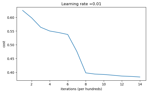
第0次迭代,成本值为:inf 第1000次迭代,成本值为:0.6250982793959966 第2000次迭代,成本值为:0.5981216596703697 第3000次迭代,成本值为:0.5638417572298645 第4000次迭代,成本值为:0.5501703049199763 第5000次迭代,成本值为:0.5444632909664456 第6000次迭代,成本值为:0.5374513807000807 第7000次迭代,成本值为:0.4764042074074983 第8000次迭代,成本值为:0.39781492295092263 第9000次迭代,成本值为:0.3934764028765484 第10000次迭代,成本值为:0.3920295461882659 第11000次迭代,成本值为:0.38924598135108 第12000次迭代,成本值为:0.3861547485712325 第13000次迭代,成本值为:0.384984728909703 第14000次迭代,成本值为:0.3827828308349524
训练集:
Accuracy: 0.83
测试集:
Accuracy: 0.86
[[1 0 1 1 0 0 1 1 1 1 1 0 1 0 0 1 0 1 1 0 0 0 1 0 1 1 1 1 1 1 0 1 1 0 0 1
  1 1 1 1 1 1 1 0 1 1 1 1 0 1 0 1 1 1 1 0 0 1 1 1 1 0 1 1 0 1 0 1 1 1 1 0
  0 0 0 0 1 0 1 0 1 1 1 0 0 1 1 1 1 1 1 0 0 1 1 1 0 1 1 0 1 0 1 1 0 1 1 0
  1 0 1 1 0 0 1 0 0 1 1 0 1 1 1 0 1 0 0 1 0 1 1 1 1 1 1 1 0 1 1 0 0 1 1 0
  0 0 1 0 1 0 1 0 1 1 1 0 0 1 1 1 1 0 1 1 0 1 0 1 1 0 1 0 1 1 1 1 0 1 1 1
  1 0 1 0 1 0 1 1 1 1 0 1 1 0 1 1 0 1 1 0 1 0 1 1 1 0 1 1 1 0 1 0 1 0 0 1
  0 1 1 0 1 1 0 1 1 0 1 1 1 0 1 1 1 1 0 1 0 0 1 1 0 1 1 1 0 0 0 1 1 0 1 1
  1 1 0 1 1 0 1 1 1 0 0 1 0 0 0 1 0 0 0 1 1 1 1 0 0 0 0 1 1 1 1 0 0 1 1 1
  1 1 1 1 0 0 0 1 1 1 1 0]]
[[1 1 1 1 0 1 0 1 1 0 1 1 1 0 0 0 0 1 0 1 0 0 1 0 1 0 1 1 1 1 1 0 0 0 0 1
  0 1 1 0 0 1 1 1 1 1 0 1 1 1 0 1 0 1 1 0 1 0 1 0 1 1 1 1 1 1 1 1 1 0 1 0
  1 1 1 1 1 0 1 0 0 1 0 0 0 1 1 0 1 1 0 0 0 1 1 0 1 1 0 0]]
我们来把图绘制出来,看看分类的结果是怎样的。
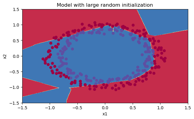
我们可以看到误差开始很高。这是因为由于具有较大的随机权重,最后一个激活(sigmoid)输出的结果非常接近于0或1,而当它出现错误时,它会导致非常高的损失。初始化参数如果没有很好地话会导致梯度消失、爆炸,这也会减慢优化算法。如果我们对这个网络进行更长时间的训练,我们将看到更好的结果,但是使用过大的随机数初始化会减慢优化的速度。
当然也可以试一试不✖10那样得到的分类情况也还不错。
我们会使用到sqrt(2/上一层的维度)这个公式来初始化参数。
def initialize_parameters_he(layers_dims):
    """
    参数:
        layers_dims - 列表,模型的层数和对应每一层的节点的数量
    返回
        parameters - 包含了所有W和b的字典
            W1 - 权重矩阵,维度为(layers_dims[1], layers_dims[0])
            b1 - 偏置向量,维度为(layers_dims[1],1)
            ···
            WL - 权重矩阵,维度为(layers_dims[L], layers_dims[L -1])
            b1 - 偏置向量,维度为(layers_dims[L],1)
    """

    np.random.seed(3)               # 指定随机种子
    parameters = {}
    L = len(layers_dims)            # 层数

    for l in range(1, L):
        parameters['W' + str(l)] = np.random.randn(layers_dims[l], layers_dims[l - 1]) * np.sqrt(2 / layers_dims[l - 1])
        parameters['b' + str(l)] = np.zeros((layers_dims[l], 1))

        #使用断言确保我的数据格式是正确的
        assert(parameters["W" + str(l)].shape == (layers_dims[l],layers_dims[l-1]))
        assert(parameters["b" + str(l)].shape == (layers_dims[l],1))

    return parameters
我们来测试一下这个函数:
parameters = initialize_parameters_he([2, 4, 1])
print("W1 = " + str(parameters["W1"]))
print("b1 = " + str(parameters["b1"]))
print("W2 = " + str(parameters["W2"]))
print("b2 = " + str(parameters["b2"]))
W1 = [[ 1.78862847 0.43650985] [ 0.09649747 -1.8634927 ] [-0.2773882 -0.35475898] [-0.08274148 -0.62700068]] b1 = [[0.] [0.] [0.] [0.]] W2 = [[-0.03098412 -0.33744411 -0.92904268 0.62552248]] b2 = [[0.]]
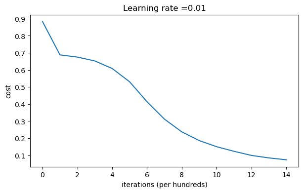
这样我们就基本把参数W初始化到了1附近,我们来实际运行一下看看:
parameters = model(train_X, train_Y, initialization = "he",is_polt=True)
print("训练集:")
predictions_train = init_utils.predict(train_X, train_Y, parameters)
print("测试集:")
init_utils.predictions_test = init_utils.predict(test_X, test_Y, parameters)
第0次迭代,成本值为:0.8830537463419761 第1000次迭代,成本值为:0.6879825919728063 第2000次迭代,成本值为:0.6751286264523371 第3000次迭代,成本值为:0.6526117768893807 第4000次迭代,成本值为:0.6082958970572937 第5000次迭代,成本值为:0.5304944491717495 第6000次迭代,成本值为:0.4138645817071793 第7000次迭代,成本值为:0.3117803464844441 第8000次迭代,成本值为:0.23696215330322556 第9000次迭代,成本值为:0.18597287209206828 第10000次迭代,成本值为:0.15015556280371808 第11000次迭代,成本值为:0.12325079292273548 第12000次迭代,成本值为:0.09917746546525937 第13000次迭代,成本值为:0.08457055954024274 第14000次迭代,成本值为:0.07357895962677366
训练集:
Accuracy: 0.9933333333333333
测试集:
Accuracy: 0.96
我们可以看到误差越来越小,我们来绘制一下预测的情况:
plt.title("Model with He initialization")
axes = plt.gca()
axes.set_xlim([-1.5, 1.5])
axes.set_ylim([-1.5, 1.5])
init_utils.plot_decision_boundary(lambda x: init_utils.predict_dec(parameters, x.T), train_X, train_Y)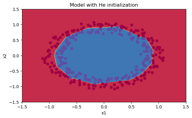
初始化的模型将蓝色和红色的点在少量的迭代中很好地分离出来
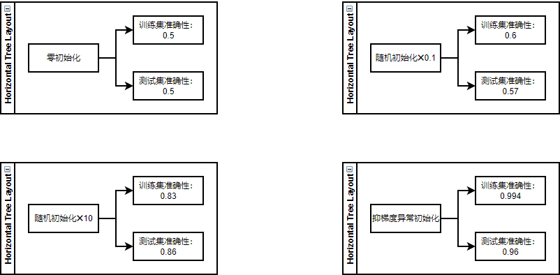
不同的初始化方法可能导致性能最终不同
随机初始化有助于打破对称,使得不同隐藏层的单元可以学习到不同的参数。
初始化时,初始值不宜过大。
He初始化搭配ReLU激活函数常常可以得到不错的效果。
接下来,我们介绍减少过拟合的方法:正则化
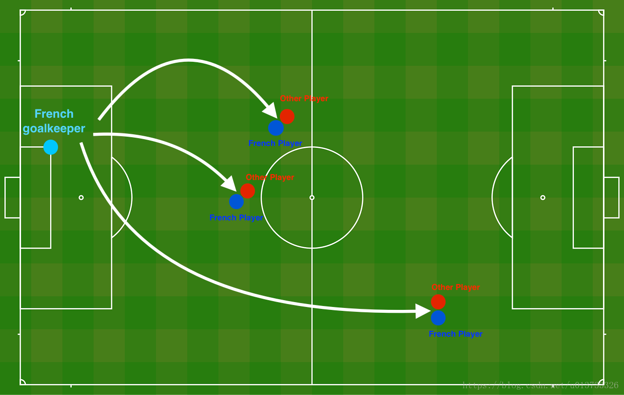
问题描述:假设你现在是一个AI专家,你需要设计一个模型,可以用于推荐在足球场中守门员将球发至哪个位置可以让本队的球员抢到球的可能性更大。
说白了,实际上就是一个二分类,一半是己方抢到球,一半就是对方抢到球,我们来看一下这个图:
train_X, train_Y, test_X, test_Y = reg_utils.load_2D_dataset(is_plot=True)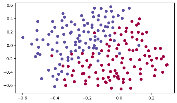
每一个点代表球落下的可能的位置,蓝色代表己方的球员会抢到球,红色代表对手的球员会抢到球,我们要做的就是使用模型来画出一条线,来找到适合我方球员能抢到球的位置。
我们要做以下三件事,来对比出不同的模型的优劣:
我们来看一下我们的模型:
def model(X,Y,learning_rate=0.3,num_iterations=30000,print_cost=True,is_plot=True,lambd=0,keep_prob=1):
    """
    实现一个三层的神经网络:LINEAR ->RELU -> LINEAR -> RELU -> LINEAR -> SIGMOID

    参数:
        X - 输入的数据,维度为(2, 要训练/测试的数量)
        Y - 标签,【0(蓝色) | 1(红色)】,维度为(1,对应的是输入的数据的标签)
        learning_rate - 学习速率
        num_iterations - 迭代的次数
        print_cost - 是否打印成本值,每迭代10000次打印一次,但是每1000次记录一个成本值
        is_polt - 是否绘制梯度下降的曲线图
        lambd - 正则化的超参数,实数
        keep_prob - 随机删除节点的概率
    返回
        parameters - 学习后的参数
    """
    grads = {}
    costs = []
    m = X.shape[1]
    layers_dims = [X.shape[0],20,3,1]

    #初始化参数
    parameters = reg_utils.initialize_parameters(layers_dims)

    #开始学习
    for i in range(0,num_iterations):
        #前向传播
        ##是否随机删除节点
        if keep_prob == 1:
            ###不随机删除节点
            a3 , cache = reg_utils.forward_propagation(X,parameters)
        elif keep_prob < 1:
            ###随机删除节点
            a3 , cache = forward_propagation_with_dropout(X,parameters,keep_prob)
        else:
            print("keep_prob参数错误!程序退出。")

        #计算成本
        ## 是否使用二范数
        if lambd == 0:
            ###不使用L2正则化
            cost = reg_utils.compute_cost(a3,Y)
        else:
            ###使用L2正则化
            cost = compute_cost_with_regularization(a3,Y,parameters,lambd)

        #反向传播
        ##可以同时使用L2正则化和随机删除节点,但是本次实验不同时使用。
        assert(lambd == 0  or keep_prob ==1)

        ##两个参数的使用情况
        if (lambd == 0 and keep_prob == 1):
            ### 不使用L2正则化和不使用随机删除节点
            grads = reg_utils.backward_propagation(X,Y,cache)
        elif (lambd != 0 and keep_prob ==1):
            ### 使用L2正则化,不使用随机删除节点
            grads = backward_propagation_with_regularization(X, Y, cache, lambd)
        elif (keep_prob < 1 and lambd ==0):
            ### 使用随机删除节点,不使用L2正则化
            grads = backward_propagation_with_dropout(X, Y, cache, keep_prob)

        #更新参数
        parameters = reg_utils.update_parameters(parameters, grads, learning_rate)

        #记录并打印成本
        if i % 1000 == 0:
            ## 记录成本
            costs.append(cost)
            if (print_cost and i % 10000 == 0):
                #打印成本
                print("第" + str(i) + "次迭代,成本值为:" + str(cost))

    #是否绘制成本曲线图
    if is_plot:
        plt.plot(costs)
        plt.ylabel('cost')
        plt.xlabel('iterations (x1,000)')
        plt.title("Learning rate =" + str(learning_rate))
        plt.show()

    #返回学习后的参数
    return parameters
我们来先看一下不使用正则化下模型的效果:
parameters = model(train_X, train_Y,is_plot=True)
print("训练集:")
predictions_train = reg_utils.predict(train_X, train_Y, parameters)
print("测试集:")
predictions_test = reg_utils.predict(test_X, test_Y, parameters)
第0次迭代,成本值为:0.6557412523481002 第10000次迭代,成本值为:0.16329987525724196 第20000次迭代,成本值为:0.13851642423253843
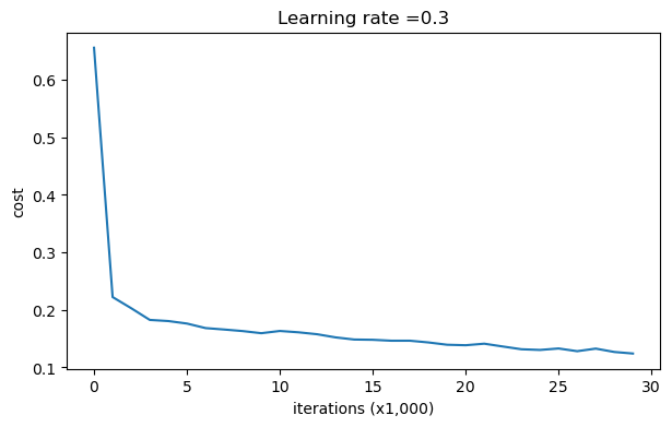
训练集:
Accuracy: 0.9478672985781991
测试集:
Accuracy: 0.915
我们可以看到,对于训练集,精确度为94%;而对于测试集,精确度为91.5%。接下来,我们将分割曲线画出来:
plt.title("Model without regularization")
axes = plt.gca()
axes.set_xlim([-0.75,0.40])
axes.set_ylim([-0.75,0.65])
reg_utils.plot_decision_boundary(lambda x: reg_utils.predict_dec(parameters, x.T), train_X, train_Y)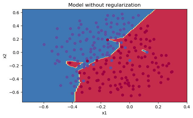
从图中可以看出,在无正则化时,分割曲线有了明显的过拟合特性。接下来,我们使用L2正则化:
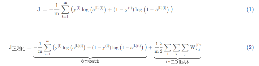
避免过度拟合的标准方法称为L2正则化,它包括适当修改你的成本函数,我们从原来的成本函数(1)到现在的函数(2):
我们下面就开始写相关的函数:
def compute_cost_with_regularization(A3,Y,parameters,lambd):
    """
    实现公式2的L2正则化计算成本

    参数:
        A3 - 正向传播的输出结果,维度为(输出节点数量,训练/测试的数量)
        Y - 标签向量,与数据一一对应,维度为(输出节点数量,训练/测试的数量)
        parameters - 包含模型学习后的参数的字典
    返回:
        cost - 使用公式2计算出来的正则化损失的值

    """
    m = Y.shape[1]
    W1 = parameters["W1"]
    W2 = parameters["W2"]
    W3 = parameters["W3"]

    cross_entropy_cost = reg_utils.compute_cost(A3,Y)

    L2_regularization_cost = lambd * (np.sum(np.square(W1)) + np.sum(np.square(W2))  + np.sum(np.square(W3))) / (2 * m)

    cost = cross_entropy_cost + L2_regularization_cost

    return cost

#当然,因为改变了成本函数,我们也必须改变向后传播的函数, 所有的梯度都必须根据这个新的成本值来计算。

def backward_propagation_with_regularization(X, Y, cache, lambd):
    """
    实现我们添加了L2正则化的模型的后向传播。

    参数:
        X - 输入数据集,维度为(输入节点数量,数据集里面的数量)
        Y - 标签,维度为(输出节点数量,数据集里面的数量)
        cache - 来自forward_propagation()的cache输出
        lambda - regularization超参数,实数

    返回:
        gradients - 一个包含了每个参数、激活值和预激活值变量的梯度的字典
    """

    m = X.shape[1]

    (Z1, A1, W1, b1, Z2, A2, W2, b2, Z3, A3, W3, b3) = cache

    dZ3 = A3 - Y

    dW3 = (1 / m) * np.dot(dZ3,A2.T) + ((lambd * W3) / m )
    db3 = (1 / m) * np.sum(dZ3,axis=1,keepdims=True)

    dA2 = np.dot(W3.T,dZ3)
    dZ2 = np.multiply(dA2,np.int64(A2 > 0)) # 应该是生成一个A2同纬度的矩阵,但是这个矩阵是A2中大于 0 的数保持不变,其余的数为 0
    dW2 = (1 / m) * np.dot(dZ2,A1.T) + ((lambd * W2) / m)
    db2 = (1 / m) * np.sum(dZ2,axis=1,keepdims=True)

    dA1 = np.dot(W2.T,dZ2)
    dZ1 = np.multiply(dA1,np.int64(A1 > 0))
    dW1 = (1 / m) * np.dot(dZ1,X.T) + ((lambd * W1) / m)
    db1 = (1 / m) * np.sum(dZ1,axis=1,keepdims=True)

    gradients = {"dZ3": dZ3, "dW3": dW3, "db3": db3, "dA2": dA2,
                 "dZ2": dZ2, "dW2": dW2, "db2": db2, "dA1": dA1,
                 "dZ1": dZ1, "dW1": dW1, "db1": db1}

    return gradients
我们来直接放到模型中跑一下:
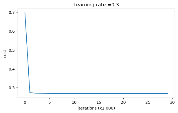
parameters = model(train_X, train_Y, lambd=0.7,is_plot=True)
print("使用正则化,训练集:")
predictions_train = reg_utils.predict(train_X, train_Y, parameters)
print("使用正则化,测试集:")
predictions_test = reg_utils.predict(test_X, test_Y, parameters)
第0次迭代,成本值为:0.6974484493131264 第10000次迭代,成本值为:0.2684918873282239 第20000次迭代,成本值为:0.2680916337127301
使用正则化,训练集:
Accuracy: 0.9383886255924171
使用正则化,测试集:
Accuracy: 0.93
我们来看一下分类的结果吧~
plt.title("Model with L2-regularization")
axes = plt.gca()
axes.set_xlim([-0.75,0.40])
axes.set_ylim([-0.75,0.65])
reg_utils.plot_decision_boundary(lambda x: reg_utils.predict_dec(parameters, x.T), train_X, train_Y)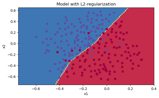
L2通过削减成本函数中权重的平方值,可以将所有权重值逐渐改变到到较小的值。权值数值高的话会有更平滑的模型,其中输入变化时输出变化更慢,但是你需要花费更多的时间。
尽管L2的速度会降低,但是它仍旧是我们减少过拟合的不二选则。
def forward_propagation_with_dropout(X,parameters,keep_prob=0.5):
"""
实现具有随机舍弃节点的前向传播。
LINEAR -> RELU + DROPOUT -> LINEAR -> RELU + DROPOUT -> LINEAR -> SIGMOID.
参数:
X - 输入数据集,维度为(2,示例数)
parameters - 包含参数“W1”,“b1”,“W2”,“b2”,“W3”,“b3”的python字典:
W1 - 权重矩阵,维度为(20,2)
b1 - 偏向量,维度为(20,1)
W2 - 权重矩阵,维度为(3,20)
b2 - 偏向量,维度为(3,1)
W3 - 权重矩阵,维度为(1,3)
b3 - 偏向量,维度为(1,1)
keep_prob - 随机删除的概率,实数
返回:
A3 - 最后的激活值,维度为(1,1),正向传播的输出
cache - 存储了一些用于计算反向传播的数值的元组
"""
np.random.seed(1)
W1 = parameters["W1"]
b1 = parameters["b1"]
W2 = parameters["W2"]
b2 = parameters["b2"]
W3 = parameters["W3"]
b3 = parameters["b3"]
#LINEAR -> RELU -> LINEAR -> RELU -> LINEAR -> SIGMOID
Z1 = np.dot(W1,X) + b1
A1 = reg_utils.relu(Z1)
#下面的步骤1-4对应于上述的步骤1-4。
D1 = np.random.rand(A1.shape[0],A1.shape[1]) #步骤1:初始化矩阵D1 = np.random.rand(..., ...)
D1 = D1 < keep_prob #步骤2:将D1的值转换为0或1(使用keep_prob作为阈值)
A1 = A1 * D1 #步骤3:舍弃A1的一些节点(将它的值变为0或False)
A1 = A1 / keep_prob #步骤4:缩放未舍弃的节点(不为0)的值
Z2 = np.dot(W2,A1) + b2
A2 = reg_utils.relu(Z2)
#下面的步骤1-4对应于上述的步骤1-4。
D2 = np.random.rand(A2.shape[0],A2.shape[1]) #步骤1:初始化矩阵D2 = np.random.rand(..., ...)
D2 = D2 < keep_prob #步骤2:将D2的值转换为0或1(使用keep_prob作为阈值)
A2 = A2 * D2 #步骤3:舍弃A1的一些节点(将它的值变为0或False)
A2 = A2 / keep_prob #步骤4:缩放未舍弃的节点(不为0)的值
Z3 = np.dot(W3, A2) + b3
A3 = reg_utils.sigmoid(Z3)
cache = (Z1, D1, A1, W1, b1, Z2, D2, A2, W2, b2, Z3, A3, W3, b3)
return A3, cache改变了前向传播的算法,我们也需要改变后向传播的算法
def backward_propagation_with_dropout(X,Y,cache,keep_prob):
    """
    实现我们随机删除的模型的后向传播。
    参数:
        X  - 输入数据集,维度为(2,示例数)
        Y  - 标签,维度为(输出节点数量,示例数量)
        cache - 来自forward_propagation_with_dropout()的cache输出
        keep_prob  - 随机删除的概率,实数

    返回:
        gradients - 一个关于每个参数、激活值和预激活变量的梯度值的字典
    """
    m = X.shape[1]
    (Z1, D1, A1, W1, b1, Z2, D2, A2, W2, b2, Z3, A3, W3, b3) = cache

    dZ3 = A3 - Y
    dW3 = (1 / m) * np.dot(dZ3,A2.T)
    db3 = 1. / m * np.sum(dZ3, axis=1, keepdims=True)
    dA2 = np.dot(W3.T, dZ3)

    dA2 = dA2 * D2          # 步骤1:使用正向传播期间相同的节点,舍弃那些关闭的节点(因为任何数乘以0或者False都为0或者False)
    dA2 = dA2 / keep_prob   # 步骤2:缩放未舍弃的节点(不为0)的值

    dZ2 = np.multiply(dA2, np.int64(A2 > 0))
    dW2 = 1. / m * np.dot(dZ2, A1.T)
    db2 = 1. / m * np.sum(dZ2, axis=1, keepdims=True)

    dA1 = np.dot(W2.T, dZ2)

    dA1 = dA1 * D1          # 步骤1:使用正向传播期间相同的节点,舍弃那些关闭的节点(因为任何数乘以0或者False都为0或者False)
    dA1 = dA1 / keep_prob   # 步骤2:缩放未舍弃的节点(不为0)的值

    dZ1 = np.multiply(dA1, np.int64(A1 > 0))
    dW1 = 1. / m * np.dot(dZ1, X.T)
    db1 = 1. / m * np.sum(dZ1, axis=1, keepdims=True)

    gradients = {"dZ3": dZ3, "dW3": dW3, "db3": db3,"dA2": dA2,
                 "dZ2": dZ2, "dW2": dW2, "db2": db2, "dA1": dA1,
                 "dZ1": dZ1, "dW1": dW1, "db1": db1}

    return gradients
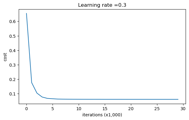
我们前向和后向传播的函数都写好了,现在用dropout运行模型(keep_prob = 0.86)跑一波。这意味着在每次迭代中,程序都可以24%的概率关闭第1层和第2层的每个神经元。调用的时候:
parameters = model(train_X, train_Y, keep_prob=0.86, learning_rate=0.3,is_plot=True)

print("使用随机删除节点,训练集:")
predictions_train = reg_utils.predict(train_X, train_Y, parameters)
print("使用随机删除节点,测试集:")
reg_utils.predictions_test = reg_utils.predict(test_X, test_Y, parameters)
第0次迭代,成本值为:0.6543912405149825
第10000次迭代,成本值为:0.061016986574905605
第20000次迭代,成本值为:0.060582435798513114
使用随机删除节点,训练集:
Accuracy: 0.9289099526066351
使用随机删除节点,测试集:
Accuracy: 0.95
我们来看看它的分类情况:
plt.title("Model with dropout")
axes = plt.gca()
axes.set_xlim([-0.75, 0.40])
axes.set_ylim([-0.75, 0.65])
reg_utils.plot_decision_boundary(lambda x: reg_utils.predict_dec(parameters, x.T), train_X, train_Y)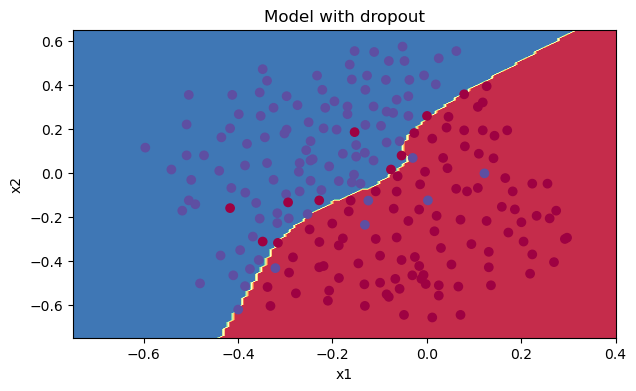
我们可以看到,正则化会把训练集的准确度降低,但是测试集的准确度提高了,所以,我们这个还是成功了。
假设你现在是一个全球移动支付团队中的一员,现在需要建立一个深度学习模型去判断用户账户在进行付款的时候是否是被黑客入侵的。
但是,在我们执行反向传播的计算过程中,反向传播函数的计算过程是比较复杂的。为了验证我们得到的反向传播函数是否正确,现在你需要编写一些代码来验证反向传播函数的正确性。
让我们回头看一下导数(或梯度)的定义:

我们先来看一下一维线性模型的梯度检查计算过程: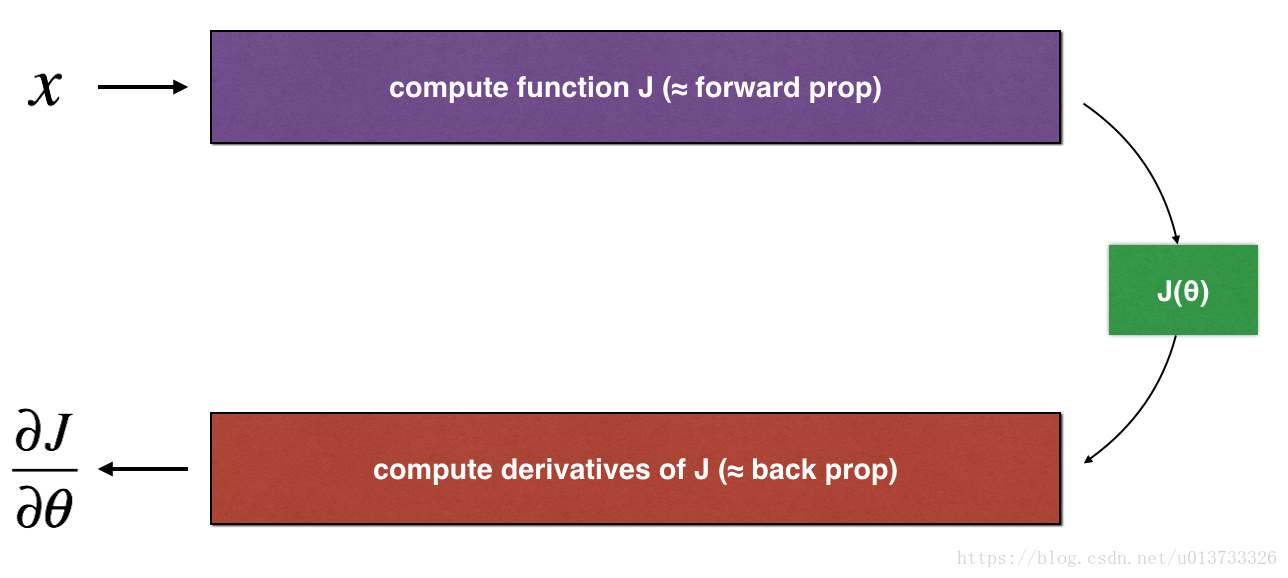
def forward_propagation(x,theta):
    """

    实现图中呈现的线性前向传播(计算J)(J(theta)= theta * x)

    参数:
    x  - 一个实值输入
    theta  - 参数,也是一个实数

    返回:
    J  - 函数J的值,用公式J(theta)= theta * x计算
    """
    J = np.dot(theta,x)

    return J
测试一下:
#测试forward_propagation
print("-----------------测试forward_propagation-----------------")
x, theta = 2, 4
J = forward_propagation(x, theta)
print ("J = " + str(J))
-----------------测试forward_propagation----------------- J = 8
前向传播有了,我们来看一下反向传播:
def backward_propagation(x,theta):
    """
    计算J相对于θ的导数。

    参数:
        x  - 一个实值输入
        theta  - 参数,也是一个实数

    返回:
        dtheta  - 相对于θ的成本梯度
    """
    dtheta = x

    return dtheta
测试一下:
#测试backward_propagation
print("-----------------测试backward_propagation-----------------")
x, theta = 2, 4
dtheta = backward_propagation(x, theta)
print ("dtheta = " + str(dtheta))
-----------------测试backward_propagation----------------- dtheta = 2
梯度检查的步骤如下:
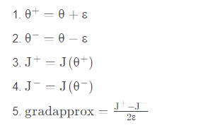
接下来,计算梯度的反向传播值,最后计算误差:

当difference小于10-7时,我们通常认为我们计算的结果是正确的。
def gradient_check(x,theta,epsilon=1e-7):
    """

    实现图中的反向传播。

    参数:
        x  - 一个实值输入
        theta  - 参数,也是一个实数
        epsilon  - 使用公式(3)计算输入的微小偏移以计算近似梯度

    返回:
        近似梯度和后向传播梯度之间的差异
    """

    #使用公式(3)的左侧计算gradapprox。
    thetaplus = theta + epsilon                               # Step 1
    thetaminus = theta - epsilon                              # Step 2
    J_plus = forward_propagation(x, thetaplus)                # Step 3
    J_minus = forward_propagation(x, thetaminus)              # Step 4
    gradapprox = (J_plus - J_minus) / (2 * epsilon)           # Step 5


    #检查gradapprox是否足够接近backward_propagation()的输出
    grad = backward_propagation(x, theta)

    numerator = np.linalg.norm(grad - gradapprox)                      # Step 1'
    denominator = np.linalg.norm(grad) + np.linalg.norm(gradapprox)    # Step 2'
    difference = numerator / denominator                               # Step 3'

    if difference < 1e-7:
        print("梯度检查:梯度正常!")
    else:
        print("梯度检查:梯度超出阈值!")

    return difference
测试一下:
#测试gradient_check
print("-----------------测试gradient_check-----------------")
x, theta = 2, 4
difference = gradient_check(x, theta)
print("difference = " + str(difference))
-----------------测试gradient_check----------------- 梯度检查:梯度正常! difference = 2.919335883291695e-10
高维参数是怎样计算的呢?我们看一下下图:
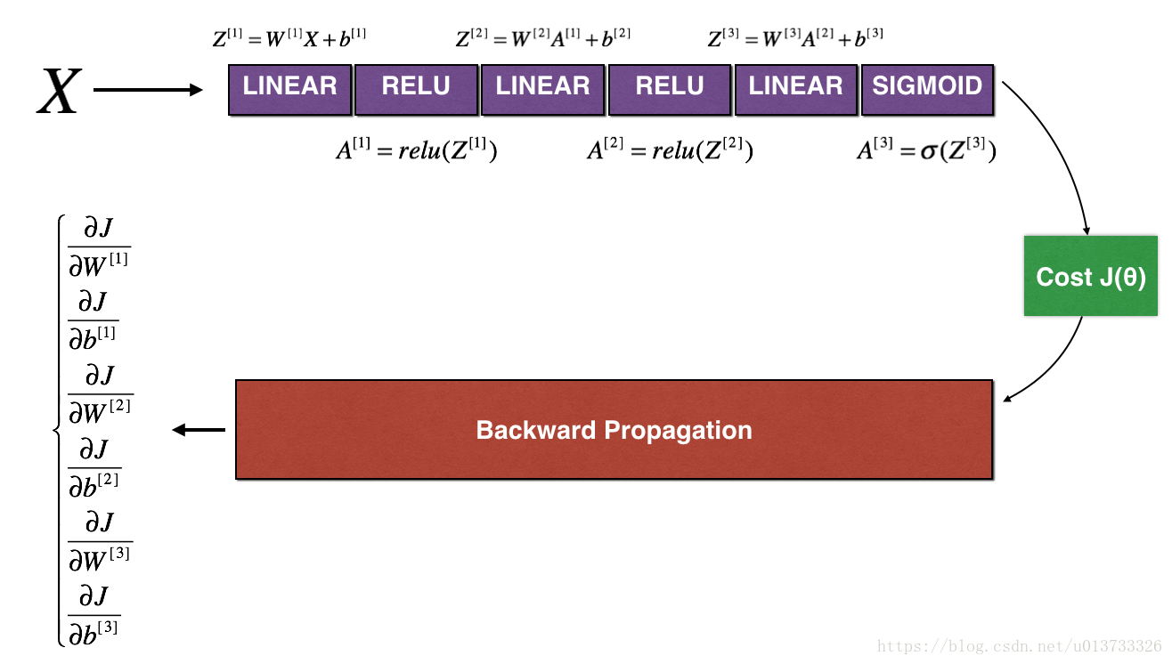
def forward_propagation_n(X,Y,parameters):
    """
    实现图中的前向传播(并计算成本)。

    参数:
        X - 训练集为m个例子
        Y -  m个示例的标签
        parameters - 包含参数“W1”,“b1”,“W2”,“b2”,“W3”,“b3”的python字典:
            W1  - 权重矩阵,维度为(5,4)
            b1  - 偏向量,维度为(5,1)
            W2  - 权重矩阵,维度为(3,5)
            b2  - 偏向量,维度为(3,1)
            W3  - 权重矩阵,维度为(1,3)
            b3  - 偏向量,维度为(1,1)

    返回:
        cost - 成本函数(logistic)
    """
    m = X.shape[1]
    W1 = parameters["W1"]
    b1 = parameters["b1"]
    W2 = parameters["W2"]
    b2 = parameters["b2"]
    W3 = parameters["W3"]
    b3 = parameters["b3"]

    # LINEAR -> RELU -> LINEAR -> RELU -> LINEAR -> SIGMOID
    Z1 = np.dot(W1,X) + b1
    A1 = gc_utils.relu(Z1)

    Z2 = np.dot(W2,A1) + b2
    A2 = gc_utils.relu(Z2)

    Z3 = np.dot(W3,A2) + b3
    A3 = gc_utils.sigmoid(Z3)

    #计算成本
    logprobs = np.multiply(-np.log(A3), Y) + np.multiply(-np.log(1 - A3), 1 - Y)
    cost = (1 / m) * np.sum(logprobs)

    cache = (Z1, A1, W1, b1, Z2, A2, W2, b2, Z3, A3, W3, b3)

    return cost, cache

def backward_propagation_n(X,Y,cache):
    """
    实现图中所示的反向传播。

    参数:
        X - 输入数据点(输入节点数量,1)
        Y - 标签
        cache - 来自forward_propagation_n()的cache输出

    返回:
        gradients - 一个字典,其中包含与每个参数、激活和激活前变量相关的成本梯度。
    """
    m = X.shape[1]
    (Z1, A1, W1, b1, Z2, A2, W2, b2, Z3, A3, W3, b3) = cache

    dZ3 = A3 - Y
    dW3 = (1. / m) * np.dot(dZ3,A2.T)
    dW3 = 1. / m * np.dot(dZ3, A2.T)
    db3 = 1. / m * np.sum(dZ3, axis=1, keepdims=True)

    dA2 = np.dot(W3.T, dZ3)
    dZ2 = np.multiply(dA2, np.int64(A2 > 0))
    #dW2 = 1. / m * np.dot(dZ2, A1.T) * 2  # Should not multiply by 2
    dW2 = 1. / m * np.dot(dZ2, A1.T)
    db2 = 1. / m * np.sum(dZ2, axis=1, keepdims=True)

    dA1 = np.dot(W2.T, dZ2)
    dZ1 = np.multiply(dA1, np.int64(A1 > 0))
    dW1 = 1. / m * np.dot(dZ1, X.T)
    #db1 = 4. / m * np.sum(dZ1, axis=1, keepdims=True) # Should not multiply by 4
    db1 = 1. / m * np.sum(dZ1, axis=1, keepdims=True)

    gradients = {"dZ3": dZ3, "dW3": dW3, "db3": db3,
                 "dA2": dA2, "dZ2": dZ2, "dW2": dW2, "db2": db2,
                 "dA1": dA1, "dZ1": dZ1, "dW1": dW1, "db1": db1}

    return gradients
然而,θ 不再是标量。 这是一个名为“parameters”的字典。 我们为你实现了一个函数“dictionary_to_vector()”。 它将“parameters”字典转换为一个称为“values”的向量,通过将所有参数(W1,b1,W2,b2,W3,b3)整形为向量并将它们连接起来而获得。
反函数是“vector_to_dictionary”,它返回“parameters”字典。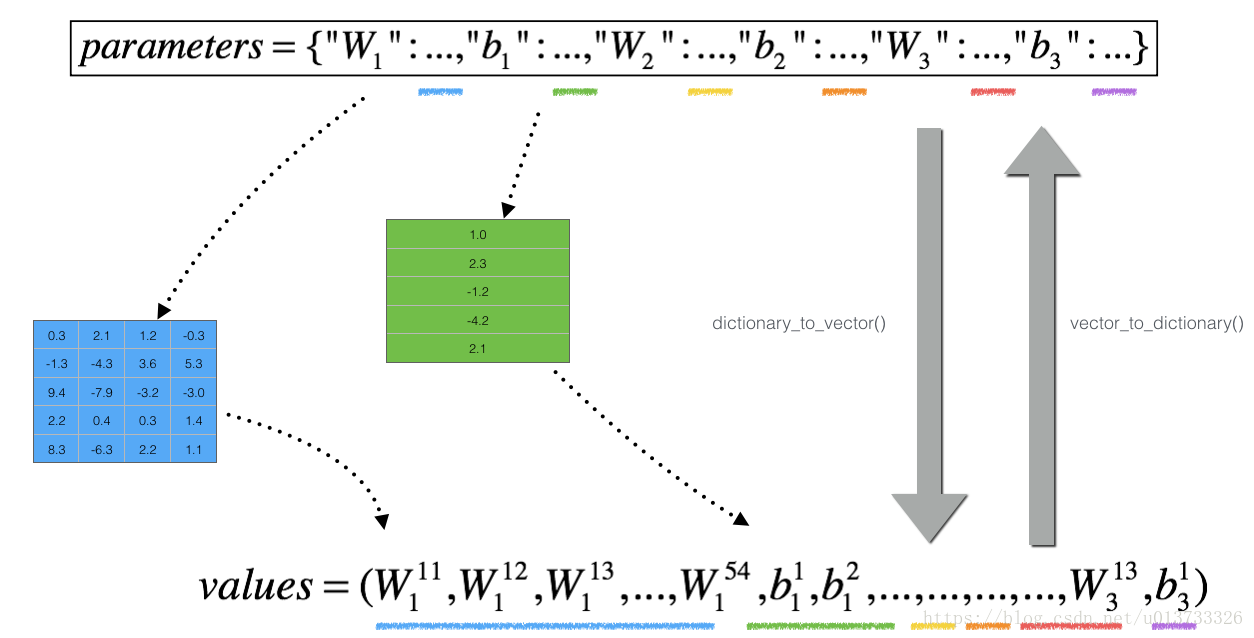
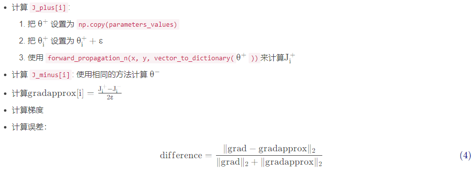
这里是伪代码,可以帮助你实现梯度检查:
def gradient_check_n(parameters,gradients,X,Y,epsilon=1e-7):
    """
    检查backward_propagation_n是否正确计算forward_propagation_n输出的成本梯度

    参数:
        parameters - 包含参数“W1”,“b1”,“W2”,“b2”,“W3”,“b3”的python字典:
        grad_output_propagation_n的输出包含与参数相关的成本梯度。
        x  - 输入数据点,维度为(输入节点数量,1)
        y  - 标签
        epsilon  - 计算输入的微小偏移以计算近似梯度

    返回:
        difference - 近似梯度和后向传播梯度之间的差异
    """
    #初始化参数
    parameters_values , keys = gc_utils.dictionary_to_vector(parameters) #keys用不到
    grad = gc_utils.gradients_to_vector(gradients)
    num_parameters = parameters_values.shape[0]
    J_plus = np.zeros((num_parameters,1))
    J_minus = np.zeros((num_parameters,1))
    gradapprox = np.zeros((num_parameters,1))

    #计算gradapprox
    for i in range(num_parameters):
        #计算J_plus [i]。输入:“parameters_values,epsilon”。输出=“J_plus [i]”
        thetaplus = np.copy(parameters_values)                                                  # Step 1
        thetaplus[i][0] = thetaplus[i][0] + epsilon                                             # Step 2
        J_plus[i], cache = forward_propagation_n(X,Y,gc_utils.vector_to_dictionary(thetaplus))  # Step 3 ,cache用不到

        #计算J_minus [i]。输入:“parameters_values,epsilon”。输出=“J_minus [i]”。
        thetaminus = np.copy(parameters_values)                                                 # Step 1
        thetaminus[i][0] = thetaminus[i][0] - epsilon                                           # Step 2
        J_minus[i], cache = forward_propagation_n(X,Y,gc_utils.vector_to_dictionary(thetaminus))# Step 3 ,cache用不到

        #计算gradapprox[i]
        gradapprox[i] = (J_plus[i] - J_minus[i]) / (2 * epsilon)

    #通过计算差异比较gradapprox和后向传播梯度。
    numerator = np.linalg.norm(grad - gradapprox)                                     # Step 1'
    denominator = np.linalg.norm(grad) + np.linalg.norm(gradapprox)                   # Step 2'
    difference = numerator / denominator                                              # Step 3'

    if difference < 1e-7:
        print("梯度检查:梯度正常!")
    else:
        print("梯度检查:梯度超出阈值!")

    return difference
检测一下:
print('=============测试梯度===============')
x,y,parameters = testCase.gradient_check_n_test_case()
cost, cache = forward_propagation_n(x,y,parameters)
gradients = backward_propagation_n(x,y,cache)
difference = gradient_check_n(parameters,gradients,x,y)
print("difference = " + str(difference))
=============测试梯度=============== 梯度检查:梯度超出阈值! difference = 1.1885552035482147e-07
到此本次课就结束了,下面是所需库的代码
# -*- coding: utf-8 -*-

#init_utils.py

import numpy as np
import matplotlib.pyplot as plt
import sklearn
import sklearn.datasets


def sigmoid(x):
    """
    Compute the sigmoid of x

    Arguments:
    x -- A scalar or numpy array of any size.

    Return:
    s -- sigmoid(x)
    """
    s = 1/(1+np.exp(-x))
    return s

def relu(x):
    """
    Compute the relu of x

    Arguments:
    x -- A scalar or numpy array of any size.

    Return:
    s -- relu(x)
    """
    s = np.maximum(0,x)

    return s

def compute_loss(a3, Y):

    """
    Implement the loss function

    Arguments:
    a3 -- post-activation, output of forward propagation
    Y -- "true" labels vector, same shape as a3

    Returns:
    loss - value of the loss function
    """

    m = Y.shape[1]
    logprobs = np.multiply(-np.log(a3),Y) + np.multiply(-np.log(1 - a3), 1 - Y)
    loss = 1./m * np.nansum(logprobs)

    return loss

def forward_propagation(X, parameters):
    """
    Implements the forward propagation (and computes the loss) presented in Figure 2.

    Arguments:
    X -- input dataset, of shape (input size, number of examples)
    Y -- true "label" vector (containing 0 if cat, 1 if non-cat)
    parameters -- python dictionary containing your parameters "W1", "b1", "W2", "b2", "W3", "b3":
                    W1 -- weight matrix of shape ()
                    b1 -- bias vector of shape ()
                    W2 -- weight matrix of shape ()
                    b2 -- bias vector of shape ()
                    W3 -- weight matrix of shape ()
                    b3 -- bias vector of shape ()

    Returns:
    loss -- the loss function (vanilla logistic loss)
    """

    # retrieve parameters
    W1 = parameters["W1"]
    b1 = parameters["b1"]
    W2 = parameters["W2"]
    b2 = parameters["b2"]
    W3 = parameters["W3"]
    b3 = parameters["b3"]

    # LINEAR -> RELU -> LINEAR -> RELU -> LINEAR -> SIGMOID
    z1 = np.dot(W1, X) + b1
    a1 = relu(z1)
    z2 = np.dot(W2, a1) + b2
    a2 = relu(z2)
    z3 = np.dot(W3, a2) + b3
    a3 = sigmoid(z3)

    cache = (z1, a1, W1, b1, z2, a2, W2, b2, z3, a3, W3, b3)

    return a3, cache

def backward_propagation(X, Y, cache):
    """
    Implement the backward propagation presented in figure 2.

    Arguments:
    X -- input dataset, of shape (input size, number of examples)
    Y -- true "label" vector (containing 0 if cat, 1 if non-cat)
    cache -- cache output from forward_propagation()

    Returns:
    gradients -- A dictionary with the gradients with respect to each parameter, activation and pre-activation variables
    """
    m = X.shape[1]
    (z1, a1, W1, b1, z2, a2, W2, b2, z3, a3, W3, b3) = cache

    dz3 = 1./m * (a3 - Y)
    dW3 = np.dot(dz3, a2.T)
    db3 = np.sum(dz3, axis=1, keepdims = True)

    da2 = np.dot(W3.T, dz3)
    dz2 = np.multiply(da2, np.int64(a2 > 0))
    dW2 = np.dot(dz2, a1.T)
    db2 = np.sum(dz2, axis=1, keepdims = True)

    da1 = np.dot(W2.T, dz2)
    dz1 = np.multiply(da1, np.int64(a1 > 0))
    dW1 = np.dot(dz1, X.T)
    db1 = np.sum(dz1, axis=1, keepdims = True)

    gradients = {"dz3": dz3, "dW3": dW3, "db3": db3,
                 "da2": da2, "dz2": dz2, "dW2": dW2, "db2": db2,
                 "da1": da1, "dz1": dz1, "dW1": dW1, "db1": db1}

    return gradients

def update_parameters(parameters, grads, learning_rate):
    """
    Update parameters using gradient descent

    Arguments:
    parameters -- python dictionary containing your parameters
    grads -- python dictionary containing your gradients, output of n_model_backward

    Returns:
    parameters -- python dictionary containing your updated parameters
                  parameters['W' + str(i)] = ...
                  parameters['b' + str(i)] = ...
    """

    L = len(parameters) // 2 # number of layers in the neural networks

    # Update rule for each parameter
    for k in range(L):
        parameters["W" + str(k+1)] = parameters["W" + str(k+1)] - learning_rate * grads["dW" + str(k+1)]
        parameters["b" + str(k+1)] = parameters["b" + str(k+1)] - learning_rate * grads["db" + str(k+1)]

    return parameters

def predict(X, y, parameters):
    """
    This function is used to predict the results of a  n-layer neural network.

    Arguments:
    X -- data set of examples you would like to label
    parameters -- parameters of the trained model

    Returns:
    p -- predictions for the given dataset X
    """

    m = X.shape[1]
    p = np.zeros((1,m), dtype = np.int)

    # Forward propagation
    a3, caches = forward_propagation(X, parameters)

    # convert probas to 0/1 predictions
    for i in range(0, a3.shape[1]):
        if a3[0,i] > 0.5:
            p[0,i] = 1
        else:
            p[0,i] = 0

    # print results
    print("Accuracy: "  + str(np.mean((p[0,:] == y[0,:]))))

    return p

def load_dataset(is_plot=True):
    np.random.seed(1)
    train_X, train_Y = sklearn.datasets.make_circles(n_samples=300, noise=.05)
    np.random.seed(2)
    test_X, test_Y = sklearn.datasets.make_circles(n_samples=100, noise=.05)
    # Visualize the data
    if is_plot:
        plt.scatter(train_X[:, 0], train_X[:, 1], c=train_Y, s=40, cmap=plt.cm.Spectral);
    train_X = train_X.T
    train_Y = train_Y.reshape((1, train_Y.shape[0]))
    test_X = test_X.T
    test_Y = test_Y.reshape((1, test_Y.shape[0]))
    return train_X, train_Y, test_X, test_Y

def plot_decision_boundary(model, X, y):
    # Set min and max values and give it some padding
    x_min, x_max = X[0, :].min() - 1, X[0, :].max() + 1
    y_min, y_max = X[1, :].min() - 1, X[1, :].max() + 1
    h = 0.01
    # Generate a grid of points with distance h between them
    xx, yy = np.meshgrid(np.arange(x_min, x_max, h), np.arange(y_min, y_max, h))
    # Predict the function value for the whole grid
    Z = model(np.c_[xx.ravel(), yy.ravel()])
    Z = Z.reshape(xx.shape)
    # Plot the contour and training examples
    plt.contourf(xx, yy, Z, cmap=plt.cm.Spectral)
    plt.ylabel('x2')
    plt.xlabel('x1')
    plt.scatter(X[0, :], X[1, :], c=y, cmap=plt.cm.Spectral)
    plt.show()

def predict_dec(parameters, X):
    """
    Used for plotting decision boundary.

    Arguments:
    parameters -- python dictionary containing your parameters
    X -- input data of size (m, K)

    Returns
    predictions -- vector of predictions of our model (red: 0 / blue: 1)
    """

    # Predict using forward propagation and a classification threshold of 0.5
    a3, cache = forward_propagation(X, parameters)
    predictions = (a3>0.5)
return predictions# -*- coding: utf-8 -*-
#gc_utils.py
import numpy as np
import matplotlib.pyplot as plt
def sigmoid(x):
"""
Compute the sigmoid of x
Arguments:
x -- A scalar or numpy array of any size.
Return:
s -- sigmoid(x)
"""
s = 1/(1+np.exp(-x))
return s
def relu(x):
"""
Compute the relu of x
Arguments:
x -- A scalar or numpy array of any size.
Return:
s -- relu(x)
"""
s = np.maximum(0,x)
return s
def dictionary_to_vector(parameters):
"""
Roll all our parameters dictionary into a single vector satisfying our specific required shape.
"""
keys = []
count = 0
for key in ["W1", "b1", "W2", "b2", "W3", "b3"]:
# flatten parameter
new_vector = np.reshape(parameters[key], (-1,1))
keys = keys + [key]*new_vector.shape[0]
if count == 0:
theta = new_vector
else:
theta = np.concatenate((theta, new_vector), axis=0)
count = count + 1
return theta, keys
def vector_to_dictionary(theta):
"""
Unroll all our parameters dictionary from a single vector satisfying our specific required shape.
"""
parameters = {}
parameters["W1"] = theta[:20].reshape((5,4))
parameters["b1"] = theta[20:25].reshape((5,1))
parameters["W2"] = theta[25:40].reshape((3,5))
parameters["b2"] = theta[40:43].reshape((3,1))
parameters["W3"] = theta[43:46].reshape((1,3))
parameters["b3"] = theta[46:47].reshape((1,1))
return parameters
def gradients_to_vector(gradients):
"""
Roll all our gradients dictionary into a single vector satisfying our specific required shape.
"""
count = 0
for key in ["dW1", "db1", "dW2", "db2", "dW3", "db3"]:
# flatten parameter
new_vector = np.reshape(gradients[key], (-1,1))
if count == 0:
theta = new_vector
else:
theta = np.concatenate((theta, new_vector), axis=0)
count = count + 1
return thetaimport numpy as np
def compute_cost_with_regularization_test_case():
np.random.seed(1)
Y_assess = np.array([[1, 1, 0, 1, 0]])
W1 = np.random.randn(2, 3)
b1 = np.random.randn(2, 1)
W2 = np.random.randn(3, 2)
b2 = np.random.randn(3, 1)
W3 = np.random.randn(1, 3)
b3 = np.random.randn(1, 1)
parameters = {"W1": W1, "b1": b1, "W2": W2, "b2": b2, "W3": W3, "b3": b3}
a3 = np.array([[ 0.40682402, 0.01629284, 0.16722898, 0.10118111, 0.40682402]])
return a3, Y_assess, parameters
def backward_propagation_with_regularization_test_case():
np.random.seed(1)
X_assess = np.random.randn(3, 5)
Y_assess = np.array([[1, 1, 0, 1, 0]])
cache = (np.array([[-1.52855314, 3.32524635, 2.13994541, 2.60700654, -0.75942115],
[-1.98043538, 4.1600994 , 0.79051021, 1.46493512, -0.45506242]]),
np.array([[ 0. , 3.32524635, 2.13994541, 2.60700654, 0. ],
[ 0. , 4.1600994 , 0.79051021, 1.46493512, 0. ]]),
np.array([[-1.09989127, -0.17242821, -0.87785842],
[ 0.04221375, 0.58281521, -1.10061918]]),
np.array([[ 1.14472371],
[ 0.90159072]]),
np.array([[ 0.53035547, 5.94892323, 2.31780174, 3.16005701, 0.53035547],
[-0.69166075, -3.47645987, -2.25194702, -2.65416996, -0.69166075],
[-0.39675353, -4.62285846, -2.61101729, -3.22874921, -0.39675353]]),
np.array([[ 0.53035547, 5.94892323, 2.31780174, 3.16005701, 0.53035547],
[ 0. , 0. , 0. , 0. , 0. ],
[ 0. , 0. , 0. , 0. , 0. ]]),
np.array([[ 0.50249434, 0.90085595],
[-0.68372786, -0.12289023],
[-0.93576943, -0.26788808]]),
np.array([[ 0.53035547],
[-0.69166075],
[-0.39675353]]),
np.array([[-0.3771104 , -4.10060224, -1.60539468, -2.18416951, -0.3771104 ]]),
np.array([[ 0.40682402, 0.01629284, 0.16722898, 0.10118111, 0.40682402]]),
np.array([[-0.6871727 , -0.84520564, -0.67124613]]),
np.array([[-0.0126646]]))
return X_assess, Y_assess, cache
def forward_propagation_with_dropout_test_case():
np.random.seed(1)
X_assess = np.random.randn(3, 5)
W1 = np.random.randn(2, 3)
b1 = np.random.randn(2, 1)
W2 = np.random.randn(3, 2)
b2 = np.random.randn(3, 1)
W3 = np.random.randn(1, 3)
b3 = np.random.randn(1, 1)
parameters = {"W1": W1, "b1": b1, "W2": W2, "b2": b2, "W3": W3, "b3": b3}
return X_assess, parameters
def backward_propagation_with_dropout_test_case():
np.random.seed(1)
X_assess = np.random.randn(3, 5)
Y_assess = np.array([[1, 1, 0, 1, 0]])
cache = (np.array([[-1.52855314, 3.32524635, 2.13994541, 2.60700654, -0.75942115],
[-1.98043538, 4.1600994 , 0.79051021, 1.46493512, -0.45506242]]), np.array([[ True, False, True, True, True],
[ True, True, True, True, False]], dtype=bool), np.array([[ 0. , 0. , 4.27989081, 5.21401307, 0. ],
[ 0. , 8.32019881, 1.58102041, 2.92987024, 0. ]]), np.array([[-1.09989127, -0.17242821, -0.87785842],
[ 0.04221375, 0.58281521, -1.10061918]]), np.array([[ 1.14472371],
[ 0.90159072]]), np.array([[ 0.53035547, 8.02565606, 4.10524802, 5.78975856, 0.53035547],
[-0.69166075, -1.71413186, -3.81223329, -4.61667916, -0.69166075],
[-0.39675353, -2.62563561, -4.82528105, -6.0607449 , -0.39675353]]), np.array([[ True, False, True, False, True],
[False, True, False, True, True],
[False, False, True, False, False]], dtype=bool), np.array([[ 1.06071093, 0. , 8.21049603, 0. , 1.06071093],
[ 0. , 0. , 0. , 0. , 0. ],
[ 0. , 0. , 0. , 0. , 0. ]]), np.array([[ 0.50249434, 0.90085595],
[-0.68372786, -0.12289023],
[-0.93576943, -0.26788808]]), np.array([[ 0.53035547],
[-0.69166075],
[-0.39675353]]), np.array([[-0.7415562 , -0.0126646 , -5.65469333, -0.0126646 , -0.7415562 ]]), np.array([[ 0.32266394, 0.49683389, 0.00348883, 0.49683389, 0.32266394]]), np.array([[-0.6871727 , -0.84520564, -0.67124613]]), np.array([[-0.0126646]]))
return X_assess, Y_assess, cache
def gradient_check_n_test_case():
np.random.seed(1)
x = np.random.randn(4,3)
y = np.array([1, 1, 0])
W1 = np.random.randn(5,4)
b1 = np.random.randn(5,1)
W2 = np.random.randn(3,5)
b2 = np.random.randn(3,1)
W3 = np.random.randn(1,3)
b3 = np.random.randn(1,1)
parameters = {"W1": W1,
"b1": b1,
"W2": W2,
"b2": b2,
"W3": W3,
"b3": b3}
return x, y, parameters
在我的gem中,我需要yaml并且在我的本地计算机上运行良好。但是在将我的gem推送到rubygems.org之后,当我尝试使用我的gem时,我收到一条错误消息=>"uninitializedconstantPsych::Syck(NameError)"谁能帮我解决这个问题?附言RubyVersion=>ruby1.9.2,GemVersion=>1.6.2,Bundlerversion=>1.0.15 最佳答案 经过几个小时的研究,我发现=>“YAML使用未维护的Syck库,而Psych使用现代的LibYAML”因此,为了解决
在我的应用程序中,我需要能够找到所有数字子字符串,然后扫描每个子字符串,找到第一个匹配范围(例如5到15之间)的子字符串,并将该实例替换为另一个字符串“X”。我的测试字符串s="1foo100bar10gee1"我的初始模式是1个或多个数字的任何字符串,例如,re=Regexp.new(/\d+/)matches=s.scan(re)给出["1","100","10","1"]如果我想用“X”替换第N个匹配项,并且只替换第N个匹配项,我该怎么做?例如,如果我想替换第三个匹配项“10”(匹配项[2]),我不能只说s[matches[2]]="X"因为它做了两次替换“1fooX0barXg
我在Rails工作并有以下类(class):classPlayer当我运行时bundleexecrailsconsole然后尝试:a=Player.new("me",5.0,"UCLA")我回来了:=>#我不知道为什么Player对象不会在这里初始化。关于可能导致此问题的操作/解释的任何建议?谢谢,马里奥格 最佳答案 havenoideawhythePlayerobjectwouldn'tbeinitializedhere它没有初始化很简单,因为你还没有初始化它!您已经覆盖了ActiveRecord::Base初始化方法,但您没有调
我有用于控制用户任务的Rails5API项目,我有以下错误,但并非总是针对相同的Controller和路由。ActionController::RoutingError:uninitializedconstantApi::V1::ApiController我向您描述了一些我的项目,以更详细地解释错误。应用结构路线scopemodule:'api'donamespace:v1do#=>Loginroutesscopemodule:'login'domatch'login',to:'sessions#login',as:'login',via::postend#=>Teamroutessc
我正在阅读一本关于Ruby的书,作者在编写类初始化定义时使用的形式与他在本书前几节中使用的形式略有不同。它看起来像这样:classTicketattr_accessor:venue,:datedefinitialize(venue,date)self.venue=venueself.date=dateendend在本书的前几节中,它的定义如下:classTicketattr_accessor:venue,:datedefinitialize(venue,date)@venue=venue@date=dateendend在第一个示例中使用setter方法与在第二个示例中使用实例变量之间是
目录前言滤波电路科普主要分类实际情况单位的概念常用评价参数函数型滤波器简单分析滤波电路构成低通滤波器RC低通滤波器RL低通滤波器高通滤波器RC高通滤波器RL高通滤波器部分摘自《LC滤波器设计与制作》,侵权删。前言最近需要学习放大电路和滤波电路,但是由于只在之前做音乐频谱分析仪的时候简单了解过一点点运放,所以也是相当从零开始学习了。滤波电路科普主要分类滤波器:主要是从不同频率的成分中提取出特定频率的信号。有源滤波器:由RC元件与运算放大器组成的滤波器。可滤除某一次或多次谐波,最普通易于采用的无源滤波器结构是将电感与电容串联,可对主要次谐波(3、5、7)构成低阻抗旁路。无源滤波器:无源滤波器,又称
最近在学习CAN,记录一下,也供大家参考交流。推荐几个我觉得很好的CAN学习,本文也是在看了他们的好文之后做的笔记首先是瑞萨的CAN入门,真的通透;秀!靠这篇我竟然2天理解了CAN协议!实战STM32F4CAN!原文链接:https://blog.csdn.net/XiaoXiaoPengBo/article/details/116206252CAN详解(小白教程)原文链接:https://blog.csdn.net/xwwwj/article/details/105372234一篇易懂的CAN通讯协议指南1一篇易懂的CAN通讯协议指南1-知乎(zhihu.com)视频推荐CAN总线个人知识总
深度学习部署:Windows安装pycocotools报错解决方法1.pycocotools库的简介2.pycocotools安装的坑3.解决办法更多Ai资讯:公主号AiCharm本系列是作者在跑一些深度学习实例时,遇到的各种各样的问题及解决办法,希望能够帮助到大家。ERROR:Commanderroredoutwithexitstatus1:'D:\Anaconda3\python.exe'-u-c'importsys,setuptools,tokenize;sys.argv[0]='"'"'C:\\Users\\46653\\AppData\\Local\\Temp\\pip-instal
@raw_array[i]=~/[\W]/非常简单的正则表达式。当我用一些非拉丁字母(具体来说是俄语)尝试时,条件是错误的。我能用它做什么? 最佳答案 @raw_array[i]=~/[\p{L}]/使用西里尔字符进行测试。引用:http://www.regular-expressions.info/unicode.html#prop 关于ruby-正则表达式将非英文字母匹配为非单词字符,我们在StackOverflow上找到一个类似的问题: https://
我需要一个非常简单的字符串验证器来显示第一个符号与所需格式不对应的位置。我想使用正则表达式,但在这种情况下,我必须找到与表达式相对应的字符串停止的位置,但我找不到可以做到这一点的方法。(这一定是一种相当简单的方法……也许没有?)例如,如果我有正则表达式:/^Q+E+R+$/带字符串:"QQQQEEE2ER"期望的结果应该是7 最佳答案 一个想法:你可以做的是标记你的模式并用可选的嵌套捕获组编写它:^(Q+(E+(R+($)?)?)?)?然后你只需要计算你获得的捕获组的数量就可以知道正则表达式引擎在模式中停止的位置,你可以确定匹配结束