PINN解偏微分方程实例1
PINN是一种利用神经网络求解偏微分方程的方法,其计算流程图如下图所示,这里以偏微分方程(1)为例。
∂
u
∂
t
+
u
∂
u
∂
x
=
v
∂
2
u
∂
x
2
\begin{align} \frac{\partial u}{\partial t}+u \frac{\partial u}{\partial x}=v\frac{\partial^2 u}{\partial x^2} \end{align}
∂t∂u+u∂x∂u=v∂x2∂2u
神经网络输入位置x,y,z和时间t的值,预测偏微分方程解u在这个时空条件下的数值解。
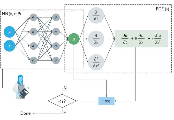
上图中可以看出,PINN的损失函数包含两部分内容,一部分是来源于训练数据误差,另一部分来源于偏微分方程误差,可以记作(2)式。
l
=
w
d
a
t
a
l
d
a
t
a
+
w
P
D
E
l
P
D
E
\begin{align} \mathcal{l} = w_{data}\mathcal{l}_{data}+w_{PDE}\mathcal{l}_{PDE} \end{align}
l=wdataldata+wPDElPDE
其中
l
d
a
t
a
=
1
N
d
a
t
a
∑
i
=
1
N
d
a
t
a
(
u
(
x
i
,
t
i
)
−
u
i
)
2
l
P
D
E
=
1
N
d
a
t
a
∑
j
=
1
N
P
D
E
(
∂
u
∂
t
+
u
∂
u
∂
x
−
v
∂
2
u
∂
x
2
)
2
∣
(
x
j
,
t
j
)
\begin{align} \begin{aligned} \mathcal{l}_{data} &= \frac{1}{N_{data}}\sum_{i=1}^{N_{data}} (u(x_i,t_i)-u_i)^2 \\ \mathcal{l}_{PDE} &= \frac{1}{N_{data}}\sum_{j=1}^{N_{PDE}} \left( \frac{\partial u}{\partial t}+u \frac{\partial u}{\partial x}-v\frac{\partial^2 u}{\partial x^2} \right)^2|_{(x_j,t_j)} \end{aligned} \end{align}
ldatalPDE=Ndata1i=1∑Ndata(u(xi,ti)−ui)2=Ndata1j=1∑NPDE(∂t∂u+u∂x∂u−v∂x2∂2u)2∣(xj,tj)
考虑偏微分方程如下:
∂
2
u
∂
x
2
−
∂
4
u
∂
y
4
=
(
2
−
x
2
)
e
−
y
\begin{align} \begin{aligned} \frac{\partial^2 u}{\partial x^2} - \frac{\partial^4 u}{\partial y^4} = (2-x^2)e^{-y} \end{aligned} \end{align}
∂x2∂2u−∂y4∂4u=(2−x2)e−y
考虑以下边界条件,
u
y
y
(
x
,
0
)
=
x
2
u
y
y
(
x
,
1
)
=
x
2
e
u
(
x
,
0
)
=
x
2
u
(
x
,
1
)
=
x
2
e
u
(
0
,
y
)
=
0
u
(
1
,
y
)
=
e
−
y
\begin{align} \begin{aligned} u_{yy}(x,0) &= x^2 \\ u_{yy}(x,1) &= \frac{x^2}{e} \\ u(x,0) &= x^2 \\ u(x,1) &= \frac{x^2}{e} \\ u(0,y) &= 0 \\ u(1,y) &= e^{-y} \\ \end{aligned} \end{align}
uyy(x,0)uyy(x,1)u(x,0)u(x,1)u(0,y)u(1,y)=x2=ex2=x2=ex2=0=e−y
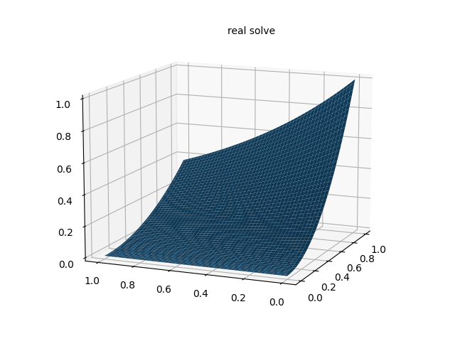
以上偏微分方程真解为
u
(
x
,
y
)
=
x
2
e
−
y
u(x,y)=x^2 e^{-y}
u(x,y)=x2e−y,在区域
[
0
,
1
]
×
[
0
,
1
]
[0,1]\times[0,1]
[0,1]×[0,1]上随机采样配置点和数据点,其中配置点用来构造PDE损失函数
l
1
,
l
2
,
⋯
,
l
7
\mathcal{l}_1,\mathcal{l}_2,\cdots,\mathcal{l}_7
l1,l2,⋯,l7,数据点用来构造数据损失函数
l
8
\mathcal{l}_8
l8.
l
1
=
1
N
1
∑
(
x
i
,
y
i
)
∈
Ω
(
u
^
x
x
(
x
i
,
y
i
;
θ
)
−
u
^
y
y
y
y
(
x
i
,
y
i
;
θ
)
−
(
2
−
x
i
2
)
e
−
y
i
)
2
l
2
=
1
N
2
∑
(
x
i
,
y
i
)
∈
[
0
,
1
]
×
{
0
}
(
u
^
y
y
(
x
i
,
y
i
;
θ
)
−
x
i
2
)
2
l
3
=
1
N
3
∑
(
x
i
,
y
i
)
∈
[
0
,
1
]
×
{
1
}
(
u
^
y
y
(
x
i
,
y
i
;
θ
)
−
x
i
2
e
)
2
l
4
=
1
N
4
∑
(
x
i
,
y
i
)
∈
[
0
,
1
]
×
{
0
}
(
u
^
(
x
i
,
y
i
;
θ
)
−
x
i
2
)
2
l
5
=
1
N
5
∑
(
x
i
,
y
i
)
∈
[
0
,
1
]
×
{
1
}
(
u
^
(
x
i
,
y
i
;
θ
)
−
x
i
2
e
)
2
l
6
=
1
N
6
∑
(
x
i
,
y
i
)
∈
{
0
}
×
[
0
,
1
]
(
u
^
(
x
i
,
y
i
;
θ
)
−
0
)
2
l
7
=
1
N
7
∑
(
x
i
,
y
i
)
∈
{
1
}
×
[
0
,
1
]
(
u
^
(
x
i
,
y
i
;
θ
)
−
e
−
y
i
)
2
l
8
=
1
N
8
∑
i
=
1
N
8
(
u
^
(
x
i
,
y
i
;
θ
)
−
u
i
)
2
\begin{align} \begin{aligned} \mathcal{l}_1 &= \frac{1}{N_1}\sum_{(x_i,y_i)\in\Omega} (\hat{u}_{xx}(x_i,y_i;\theta) - \hat{u}_{yyyy}(x_i,y_i;\theta) - (2-x_i^2)e^{-y_i})^2 \\ \mathcal{l}_2 &= \frac{1}{N_2}\sum_{(x_i,y_i)\in[0,1]\times\{0\}} (\hat{u}_{yy}(x_i,y_i;\theta) - x_i^2)^2 \\ \mathcal{l}_3 &= \frac{1}{N_3}\sum_{(x_i,y_i)\in[0,1]\times\{1\}} (\hat{u}_{yy}(x_i,y_i;\theta) - \frac{x_i^2}{e})^2 \\ \mathcal{l}_4 &= \frac{1}{N_4}\sum_{(x_i,y_i)\in[0,1]\times\{0\}} (\hat{u}(x_i,y_i;\theta) - x_i^2)^2 \\ \mathcal{l}_5 &= \frac{1}{N_5}\sum_{(x_i,y_i)\in[0,1]\times\{1\}} (\hat{u}(x_i,y_i;\theta) - \frac{x_i^2}{e})^2 \\ \mathcal{l}_6 &= \frac{1}{N_6}\sum_{(x_i,y_i)\in\{0\}\times [0,1]}(\hat{u}(x_i,y_i;\theta) - 0)^2 \\ \mathcal{l}_7 &= \frac{1}{N_7}\sum_{(x_i,y_i)\in\{1\}\times [0,1]}(\hat{u}(x_i,y_i;\theta) - e^{-y_i})^2 \\ \mathcal{l}_8 &= \frac{1}{N_{8}}\sum_{i=1}^{N_{8}} (\hat{u}(x_i,y_i;\theta)-u_i)^2 \end{aligned} \end{align}
l1l2l3l4l5l6l7l8=N11(xi,yi)∈Ω∑(u^xx(xi,yi;θ)−u^yyyy(xi,yi;θ)−(2−xi2)e−yi)2=N21(xi,yi)∈[0,1]×{0}∑(u^yy(xi,yi;θ)−xi2)2=N31(xi,yi)∈[0,1]×{1}∑(u^yy(xi,yi;θ)−exi2)2=N41(xi,yi)∈[0,1]×{0}∑(u^(xi,yi;θ)−xi2)2=N51(xi,yi)∈[0,1]×{1}∑(u^(xi,yi;θ)−exi2)2=N61(xi,yi)∈{0}×[0,1]∑(u^(xi,yi;θ)−0)2=N71(xi,yi)∈{1}×[0,1]∑(u^(xi,yi;θ)−e−yi)2=N81i=1∑N8(u^(xi,yi;θ)−ui)2
"""
A scratch for PINN solving the following PDE
u_xx-u_yyyy=(2-x^2)*exp(-y)
Author: ST
Date: 2023/2/26
"""
import torch
import matplotlib.pyplot as plt
from mpl_toolkits.mplot3d import Axes3D
epochs = 10000 # 训练代数
h = 100 # 画图网格密度
N = 1000 # 内点配置点数
N1 = 100 # 边界点配置点数
N2 = 1000 # PDE数据点
def setup_seed(seed):
torch.manual_seed(seed)
torch.cuda.manual_seed_all(seed)
torch.backends.cudnn.deterministic = True
# 设置随机数种子
setup_seed(888888)
# Domain and Sampling
def interior(n=N):
# 内点
x = torch.rand(n, 1)
y = torch.rand(n, 1)
cond = (2 - x ** 2) * torch.exp(-y)
return x.requires_grad_(True), y.requires_grad_(True), cond
def down_yy(n=N1):
# 边界 u_yy(x,0)=x^2
x = torch.rand(n, 1)
y = torch.zeros_like(x)
cond = x ** 2
return x.requires_grad_(True), y.requires_grad_(True), cond
def up_yy(n=N1):
# 边界 u_yy(x,1)=x^2/e
x = torch.rand(n, 1)
y = torch.ones_like(x)
cond = x ** 2 / torch.e
return x.requires_grad_(True), y.requires_grad_(True), cond
def down(n=N1):
# 边界 u(x,0)=x^2
x = torch.rand(n, 1)
y = torch.zeros_like(x)
cond = x ** 2
return x.requires_grad_(True), y.requires_grad_(True), cond
def up(n=N1):
# 边界 u(x,1)=x^2/e
x = torch.rand(n, 1)
y = torch.ones_like(x)
cond = x ** 2 / torch.e
return x.requires_grad_(True), y.requires_grad_(True), cond
def left(n=N1):
# 边界 u(0,y)=0
y = torch.rand(n, 1)
x = torch.zeros_like(y)
cond = torch.zeros_like(x)
return x.requires_grad_(True), y.requires_grad_(True), cond
def right(n=N1):
# 边界 u(1,y)=e^(-y)
y = torch.rand(n, 1)
x = torch.ones_like(y)
cond = torch.exp(-y)
return x.requires_grad_(True), y.requires_grad_(True), cond
def data_interior(n=N2):
# 内点
x = torch.rand(n, 1)
y = torch.rand(n, 1)
cond = (x ** 2) * torch.exp(-y)
return x.requires_grad_(True), y.requires_grad_(True), cond
# Neural Network
class MLP(torch.nn.Module):
def __init__(self):
super(MLP, self).__init__()
self.net = torch.nn.Sequential(
torch.nn.Linear(2, 32),
torch.nn.Tanh(),
torch.nn.Linear(32, 32),
torch.nn.Tanh(),
torch.nn.Linear(32, 32),
torch.nn.Tanh(),
torch.nn.Linear(32, 32),
torch.nn.Tanh(),
torch.nn.Linear(32, 1)
)
def forward(self, x):
return self.net(x)
# Loss
loss = torch.nn.MSELoss()
def gradients(u, x, order=1):
if order == 1:
return torch.autograd.grad(u, x, grad_outputs=torch.ones_like(u),
create_graph=True,
only_inputs=True, )[0]
else:
return gradients(gradients(u, x), x, order=order - 1)
# 以下7个损失是PDE损失
def l_interior(u):
# 损失函数L1
x, y, cond = interior()
uxy = u(torch.cat([x, y], dim=1))
return loss(gradients(uxy, x, 2) - gradients(uxy, y, 4), cond)
def l_down_yy(u):
# 损失函数L2
x, y, cond = down_yy()
uxy = u(torch.cat([x, y], dim=1))
return loss(gradients(uxy, y, 2), cond)
def l_up_yy(u):
# 损失函数L3
x, y, cond = up_yy()
uxy = u(torch.cat([x, y], dim=1))
return loss(gradients(uxy, y, 2), cond)
def l_down(u):
# 损失函数L4
x, y, cond = down()
uxy = u(torch.cat([x, y], dim=1))
return loss(uxy, cond)
def l_up(u):
# 损失函数L5
x, y, cond = up()
uxy = u(torch.cat([x, y], dim=1))
return loss(uxy, cond)
def l_left(u):
# 损失函数L6
x, y, cond = left()
uxy = u(torch.cat([x, y], dim=1))
return loss(uxy, cond)
def l_right(u):
# 损失函数L7
x, y, cond = right()
uxy = u(torch.cat([x, y], dim=1))
return loss(uxy, cond)
# 构造数据损失
def l_data(u):
# 损失函数L8
x, y, cond = data_interior()
uxy = u(torch.cat([x, y], dim=1))
return loss(uxy, cond)
# Training
u = MLP()
opt = torch.optim.Adam(params=u.parameters())
for i in range(epochs):
opt.zero_grad()
l = l_interior(u) \
+ l_up_yy(u) \
+ l_down_yy(u) \
+ l_up(u) \
+ l_down(u) \
+ l_left(u) \
+ l_right(u) \
+ l_data(u)
l.backward()
opt.step()
if i % 100 == 0:
print(i)
# Inference
xc = torch.linspace(0, 1, h)
xm, ym = torch.meshgrid(xc, xc)
xx = xm.reshape(-1, 1)
yy = ym.reshape(-1, 1)
xy = torch.cat([xx, yy], dim=1)
u_pred = u(xy)
u_real = xx * xx * torch.exp(-yy)
u_error = torch.abs(u_pred-u_real)
u_pred_fig = u_pred.reshape(h,h)
u_real_fig = u_real.reshape(h,h)
u_error_fig = u_error.reshape(h,h)
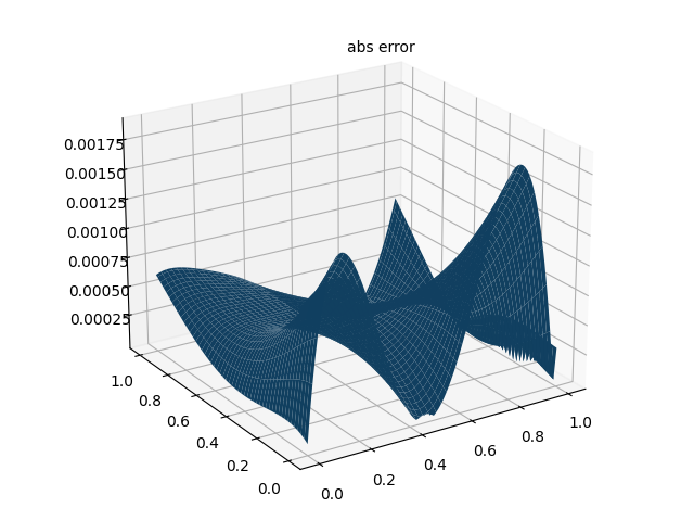
print("Max abs error is: ", float(torch.max(torch.abs(u_pred - xx * xx * torch.exp(-yy)))))
# 仅有PDE损失 Max abs error: 0.004852950572967529
# 带有数据点损失 Max abs error: 0.0018916130065917969
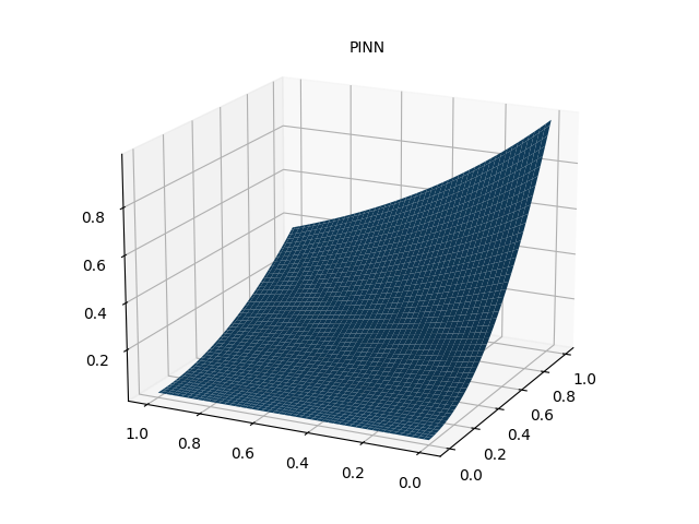
# 作PINN数值解图
fig = plt.figure()
ax = Axes3D(fig)
ax.plot_surface(xm.detach().numpy(), ym.detach().numpy(), u_pred_fig.detach().numpy())
ax.text2D(0.5, 0.9, "PINN", transform=ax.transAxes)
plt.show()
fig.savefig("PINN solve.png")
# 作真解图
fig = plt.figure()
ax = Axes3D(fig)
ax.plot_surface(xm.detach().numpy(), ym.detach().numpy(), u_real_fig.detach().numpy())
ax.text2D(0.5, 0.9, "real solve", transform=ax.transAxes)
plt.show()
fig.savefig("real solve.png")
# 误差图
fig = plt.figure()
ax = Axes3D(fig)
ax.plot_surface(xm.detach().numpy(), ym.detach().numpy(), u_error_fig.detach().numpy())
ax.text2D(0.5, 0.9, "abs error", transform=ax.transAxes)
plt.show()
fig.savefig("abs error.png")
我正在查看instance_variable_set的文档并看到给出的示例代码是这样做的:obj.instance_variable_set(:@instnc_var,"valuefortheinstancevariable")然后允许您在类的任何实例方法中以@instnc_var的形式访问该变量。我想知道为什么在@instnc_var之前需要一个冒号:。冒号有什么作用? 最佳答案 我的第一直觉是告诉你不要使用instance_variable_set除非你真的知道你用它做什么。它本质上是一种元编程工具或绕过实例变量可见性的黑客攻击
在我的应用程序中,我需要能够找到所有数字子字符串,然后扫描每个子字符串,找到第一个匹配范围(例如5到15之间)的子字符串,并将该实例替换为另一个字符串“X”。我的测试字符串s="1foo100bar10gee1"我的初始模式是1个或多个数字的任何字符串,例如,re=Regexp.new(/\d+/)matches=s.scan(re)给出["1","100","10","1"]如果我想用“X”替换第N个匹配项,并且只替换第N个匹配项,我该怎么做?例如,如果我想替换第三个匹配项“10”(匹配项[2]),我不能只说s[matches[2]]="X"因为它做了两次替换“1fooX0barXg
我有一个正在构建的应用程序,我需要一个模型来创建另一个模型的实例。我希望每辆车都有4个轮胎。汽车模型classCar轮胎模型classTire但是,在make_tires内部有一个错误,如果我为Tire尝试它,则没有用于创建或新建的activerecord方法。当我检查轮胎时,它没有这些方法。我该如何补救?错误是这样的:未定义的方法'create'forActiveRecord::AttributeMethods::Serialization::Tire::Module我测试了两个环境:测试和开发,它们都因相同的错误而失败。 最佳答案
我正在处理旧代码的一部分。beforedoallow_any_instance_of(SportRateManager).toreceive(:create).and_return(true)endRubocop错误如下:Avoidstubbingusing'allow_any_instance_of'我读到了RuboCop::RSpec:AnyInstance我试着像下面那样改变它。由此beforedoallow_any_instance_of(SportRateManager).toreceive(:create).and_return(true)end对此:let(:sport_
我收到格式为的回复#我需要将其转换为哈希值(针对活跃商家)。目前我正在遍历变量并执行此操作:response.instance_variables.eachdo|r|my_hash.merge!(r.to_s.delete("@").intern=>response.instance_eval(r.to_s.delete("@")))end这有效,它将生成{:first="charlie",:last=>"kelly"},但它似乎有点hacky和不稳定。有更好的方法吗?编辑:我刚刚意识到我可以使用instance_variable_get作为该等式的第二部分,但这仍然是主要问题。
为什么以下不同?Time.now.end_of_day==Time.now.end_of_day-0.days#falseTime.now.end_of_day.to_s==Time.now.end_of_day-0.days.to_s#true 最佳答案 因为纳秒数不同:ruby-1.9.2-p180:014>(Time.now.end_of_day-0.days).nsec=>999999000ruby-1.9.2-p180:015>Time.now.end_of_day.nsec=>999999998
我正在写一篇关于在Ruby中几乎一切都是对象的博客文章,我试图通过以下示例来展示这一点:classCoolBeansattr_accessor:beansdefinitialize@bean=[]enddefcount_beans@beans.countendend所以从类中我们可以看出它有4个方法(当然,除非我错了):它可以在创建新实例时初始化一个默认的空bean数组它可以计算它有多少个bean它可以读取它有多少个bean(通过attr_accessor)它可以向空数组写入(或添加)更多bean(也通过attr_accessor)但是,当我询问类本身它有哪些实例方法时,我没有看到默认
如果我有以下一段Ruby代码:classBlahdefself.bleh@blih="Hello"@@bloh="World"endend@blih和@@bloh到底是什么?@blih是Blah类中的一个实例变量,@@bloh是Blah类中的一个类变量,对吗?这是否意味着@@bloh是Blah的类Class中的一个变量? 最佳答案 人们似乎忽略了该方法是类方法。@blih将是常量Bleh的类Class实例的实例变量。因此:irb(main):001:0>classBlehirb(main):002:1>defself.blehirb
我理解(我认为)Ruby中类变量和类的实例变量之间的区别。我想知道如何从该类外部访问该类的实例变量。从内部(即在类方法中而不是实例方法中),它可以直接访问,但是从外部,有没有办法做MyClass.class.[@$#]variablename?我没有任何具体原因要这样做,只是学习Ruby并想知道是否可行。 最佳答案 classMyClass@my_class_instance_var="foo"class上述yield:>>foo我相信Arkku演示了如何从类外部访问类变量(@@),而不是类实例变量(@)。我从这篇文章中提取了上述内
print"Enteryourpassword:"pass=STDIN.noecho(&:gets)puts"Yourpasswordis#{pass}!"输出:Enteryourpassword:input.rb:2:in`':undefinedmethod`noecho'for#>(NoMethodError) 最佳答案 一开始require'io/console'后来的Ruby1.9.3 关于ruby-为什么不能使用类IO的实例方法noecho?,我们在StackOverflow上