本文介绍基于Python语言中TensorFlow的Keras接口,实现深度神经网络回归的方法。
前期一篇文章Python TensorFlow深度学习回归代码:DNNRegressor详细介绍了基于TensorFlow tf.estimator接口的深度学习网络;而在TensorFlow 2.0中,新的Keras接口具有与 tf.estimator接口一致的功能,且其更易于学习,对于新手而言友好程度更高;在TensorFlow官网也建议新手从Keras接口入手开始学习。因此,本文结合TensorFlow Keras接口,加以深度学习回归的详细介绍与代码实战。
和上述博客类似,本文第二部分为代码的分解介绍,第三部分为完整代码。一些在上述博客介绍过的内容,在本文中就省略了,大家如果有需要可以先查看上述文章Python TensorFlow深度学习回归代码:DNNRegressor。
相关版本信息:Python版本:3.8.5;TensorFlow版本:2.4.1;编译器版本:Spyder 4.1.5。
首先需要引入相关的库与包。
import os
import glob
import openpyxl
import numpy as np
import pandas as pd
import seaborn as sns
import tensorflow as tf
import scipy.stats as stats
import matplotlib.pyplot as plt
from sklearn import metrics
from tensorflow import keras
from tensorflow.keras import layers
from tensorflow.keras import regularizers
from tensorflow.keras.callbacks import ModelCheckpoint
from tensorflow.keras.layers.experimental import preprocessing
由于后续代码执行过程中,会有很多数据的展示与输出,其中多数数据都带有小数部分;为了让程序所显示的数据更为整齐、规范,我们可以对代码的浮点数、数组与NumPy对象对应的显示规则加以约束。
np.set_printoptions(precision=4,suppress=True)
其中,precision设置小数点后显示的位数,默认为8;suppress表示是否使用定点计数法(即与科学计数法相对)。
深度学习代码一大特点即为具有较多的参数需要我们手动定义。为避免调参时上下翻找,我们可以将主要的参数集中在一起,方便我们后期调整。
其中,具体参数的含义在本文后续部分详细介绍。
# Input parameters.
DataPath="G:/CropYield/03_DL/00_Data/AllDataAll.csv"
ModelPath="G:/CropYield/03_DL/02_DNNModle"
CheckPointPath="G:/CropYield/03_DL/02_DNNModle/Weights"
CheckPointName=CheckPointPath+"/Weights_{epoch:03d}_{val_loss:.4f}.hdf5"
ParameterPath="G:/CropYield/03_DL/03_OtherResult/ParameterResult.xlsx"
TrainFrac=0.8
RandomSeed=np.random.randint(low=21,high=22)
CheckPointMethod='val_loss'
HiddenLayer=[64,128,256,512,512,1024,1024]
RegularizationFactor=0.0001
ActivationMethod='relu'
DropoutValue=[0.5,0.5,0.5,0.3,0.3,0.3,0.2]
OutputLayerActMethod='linear'
LossMethod='mean_absolute_error'
LearnRate=0.005
LearnDecay=0.0005
FitEpoch=500
BatchSize=9999
ValFrac=0.2
BestEpochOptMethod='adam'
我的数据已经保存在了.csv文件中,因此可以用pd.read_csv直接读取。
其中,数据的每一列是一个特征,每一行是全部特征与因变量(就是下面的Yield)组合成的样本。
# Fetch and divide data.
MyData=pd.read_csv(DataPath,names=['EVI0610','EVI0626','EVI0712','EVI0728','EVI0813','EVI0829',
                                   'EVI0914','EVI0930','EVI1016','Lrad06','Lrad07','Lrad08',
                                   'Lrad09','Lrad10','Prec06','Prec07','Prec08','Prec09',
                                   'Prec10','Pres06','Pres07','Pres08','Pres09','Pres10',
                                   'SIF161','SIF177','SIF193','SIF209','SIF225','SIF241',
                                   'SIF257','SIF273','SIF289','Shum06','Shum07','Shum08',
                                   'Shum09','Shum10','SoilType','Srad06','Srad07','Srad08',
                                   'Srad09','Srad10','Temp06','Temp07','Temp08','Temp09',
                                   'Temp10','Wind06','Wind07','Wind08','Wind09','Wind10',
                                   'Yield'],header=0)
随后,对导入的数据划分训练集与测试集。
TrainData=MyData.sample(frac=TrainFrac,random_state=RandomSeed)
TestData=MyData.drop(TrainData.index)
其中,TrainFrac为训练集(包括验证数据)所占比例,RandomSeed为随即划分数据时所用的随机数种子。
在开始深度学习前,我们可以分别对输入数据的不同特征与因变量的关系加以查看。绘制联合分布图就是一种比较好的查看多个变量之间关系的方法。我们用seaborn来实现这一过程。seaborn是一个基于matplotlib的Python数据可视化库,使得我们可以通过较为简单的操作,绘制出动人的图片。代码如下:
# Draw the joint distribution image.
def JointDistribution(Factors):
    plt.figure(1)
    sns.pairplot(TrainData[Factors],kind='reg',diag_kind='kde')
    sns.set(font_scale=2.0)
    DataDistribution=TrainData.describe().transpose()

# Draw the joint distribution image.
JointFactor=['Lrad07','Prec06','SIF161','Shum06','Srad07','Srad08','Srad10','Temp06','Yield']
JointDistribution(JointFactor)
其中,JointFactor为需要绘制联合分布图的特征名称,JointDistribution函数中的kind表示联合分布图中非对角线图的类型,可选'reg'与'scatter'、'kde'、'hist','reg'代表在图片中加入一条拟合直线,'scatter'就是不加入这条直线,'kde'是等高线的形式,'hist'就是类似于栅格地图的形式;diag_kind表示联合分布图中对角线图的类型,可选'hist'与'kde','hist'代表直方图,'kde'代表直方图曲线化。font_scale是图中的字体大小。JointDistribution函数中最后一句是用来展示TrainData中每一项特征数据的统计信息,包括最大值、最小值、平均值、分位数等。
图片绘制的示例如下:
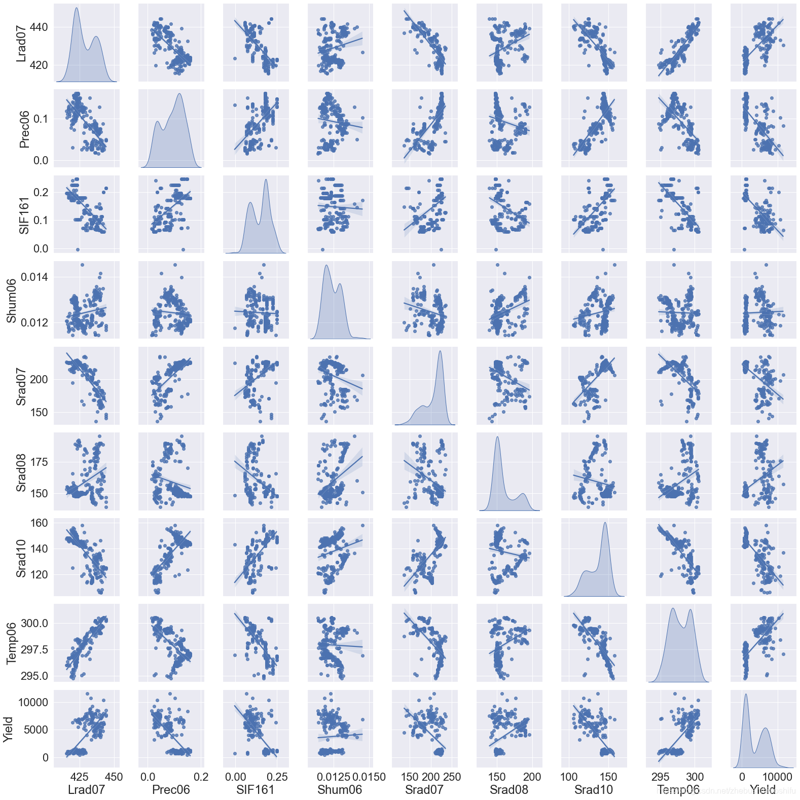
要注意,绘制联合分布图比较慢,建议大家不要选取太多的变量,否则程序会卡在这里比较长的时间。
因变量分离我们就不再多解释啦;接下来,我们要知道,对于机器学习、深度学习而言,数据标准化是十分重要的——用官网所举的一个例子:不同的特征在神经网络中会乘以相同的权重weight,因此输入数据的尺度(即数据不同特征之间的大小关系)将会影响到输出数据与梯度的尺度;因此,数据标准化可以使得模型更加稳定。
在这里,首先说明数据标准化与归一化的区别。
标准化即将训练集中某列的值缩放成均值为0,方差为1的状态;而归一化是将训练集中某列的值缩放到0和1之间。而在机器学习中,标准化较之归一化通常具有更高的使用频率,且标准化后的数据在神经网络训练时,其收敛将会更快。
最后,一定要记得——标准化时只需要对训练集数据加以处理,不要把测试集Test的数据引入了!因为标准化只需要对训练数据加以处理,引入测试集反而会影响标准化的作用。
# Separate independent and dependent variables.
TrainX=TrainData.copy(deep=True)
TestX=TestData.copy(deep=True)
TrainY=TrainX.pop('Yield')
TestY=TestX.pop('Yield')

# Standardization data.
Normalizer=preprocessing.Normalization()
Normalizer.adapt(np.array(TrainX))
在这里,我们直接运用preprocessing.Normalization()建立一个预处理层,其具有数据标准化的功能;随后,通过.adapt()函数将需要标准化的数据(即训练集的自变量)放入这一层,便可以实现数据的标准化操作。
我们的程序每执行一次,便会在指定路径中保存当前运行的模型。为保证下一次模型保存时不受上一次模型运行结果干扰,我们可以将模型文件夹内的全部文件删除。
# Delete the model result from the last run.
def DeleteOldModel(ModelPath):
    AllFileName=os.listdir(ModelPath)
    for i in AllFileName:
        NewPath=os.path.join(ModelPath,i)
        if os.path.isdir(NewPath):
            DeleteOldModel(NewPath)
        else:
            os.remove(NewPath)

# Delete the model result from the last run.
DeleteOldModel(ModelPath)
这一部分的代码在文章Python TensorFlow深度学习回归代码:DNNRegressor有详细的讲解,这里就不再重复。
在我们训练模型的过程中,会让模型运行几百个Epoch(一个Epoch即全部训练集数据样本均进入模型训练一次);而由于每一次的Epoch所得到的精度都不一样,那么我们自然需要挑出几百个Epoch中最优秀的那一个Epoch。
# Find and save optimal epoch.
def CheckPoint(Name):
    Checkpoint=ModelCheckpoint(Name,
                               monitor=CheckPointMethod,
                               verbose=1,
                               save_best_only=True,
                               mode='auto')
    CallBackList=[Checkpoint]
    return CallBackList

# Find and save optimal epochs.
CallBack=CheckPoint(CheckPointName)
其中,Name就是保存Epoch的路径与文件名命名方法;monitor是我们挑选最优Epoch的依据,在这里我们用验证集数据对应的误差来判断这个Epoch是不是我们想要的;verbose用来设置输出日志的内容,我们用1就好;save_best_only用来确定我们是否只保存被认定为最优的Epoch;mode用以判断我们的monitor是越大越好还是越小越好,前面提到了我们的monitor是验证集数据对应的误差,那么肯定是误差越小越好,所以这里可以用'auto'或'min',其中'auto'是模型自己根据用户选择的monitor方法来判断越大越好还是越小越好。
找到最优Epoch后,将其传递给CallBack。需要注意的是,这里的最优Epoch是多个Epoch——因为每一次Epoch只要获得了当前模型所遇到的最优解,它就会保存;下一次再遇见一个更好的解时,同样保存,且不覆盖上一次的Epoch。可以这么理解,假如一共有三次Epoch,所得到的误差分别为5,7,4;那么我们保存的Epoch就是第一次和第三次。
Keras接口下的模型构建就很清晰明了了。相信大家在看了前期一篇文章Python TensorFlow深度学习回归代码:DNNRegressor后,结合代码旁的注释就理解啦。
# Build DNN model.
def BuildModel(Norm):
    Model=keras.Sequential([Norm, # 数据标准化层

                            layers.Dense(HiddenLayer[0], # 指定隐藏层1的神经元个数
                                         kernel_regularizer=regularizers.l2(RegularizationFactor), # 运用L2正则化
                                         # activation=ActivationMethod
                                         ),
                            layers.LeakyReLU(), # 引入LeakyReLU这一改良的ReLU激活函数,从而加快模型收敛,减少过拟合
                            layers.BatchNormalization(), # 引入Batch Normalizing,加快网络收敛与增强网络稳固性
                            layers.Dropout(DropoutValue[0]), # 指定隐藏层1的Dropout值

                            layers.Dense(HiddenLayer[1],
                                         kernel_regularizer=regularizers.l2(RegularizationFactor),
                                         # activation=ActivationMethod
                                         ),
                            layers.LeakyReLU(),
                            layers.BatchNormalization(),
                            layers.Dropout(DropoutValue[1]),

                            layers.Dense(HiddenLayer[2],
                                         kernel_regularizer=regularizers.l2(RegularizationFactor),
                                         # activation=ActivationMethod
                                         ),
                            layers.LeakyReLU(),
                            layers.BatchNormalization(),
                            layers.Dropout(DropoutValue[2]),

                            layers.Dense(HiddenLayer[3],
                                         kernel_regularizer=regularizers.l2(RegularizationFactor),
                                         # activation=ActivationMethod
                                         ),
                            layers.LeakyReLU(),
                            layers.BatchNormalization(),
                            layers.Dropout(DropoutValue[3]),

                            layers.Dense(HiddenLayer[4],
                                         kernel_regularizer=regularizers.l2(RegularizationFactor),
                                         # activation=ActivationMethod
                                         ),
                            layers.LeakyReLU(),
                            layers.BatchNormalization(),
                            layers.Dropout(DropoutValue[4]),

                            layers.Dense(HiddenLayer[5],
                                         kernel_regularizer=regularizers.l2(RegularizationFactor),
                                         # activation=ActivationMethod
                                         ),
                            layers.LeakyReLU(),
                            layers.BatchNormalization(),
                            layers.Dropout(DropoutValue[5]),

                            layers.Dense(HiddenLayer[6],
                                         kernel_regularizer=regularizers.l2(RegularizationFactor),
                                         # activation=ActivationMethod
                                         ),
                            layers.LeakyReLU(),
                            # If batch normalization is set in the last hidden layer, the error image
                            # will show a trend of first stable and then decline; otherwise, it will
                            # decline and then stable.
                            # layers.BatchNormalization(),
                            layers.Dropout(DropoutValue[6]),

                            layers.Dense(units=1,
                                         activation=OutputLayerActMethod)]) # 最后一层就是输出层
    Model.compile(loss=LossMethod, # 指定每个批次训练误差的减小方法
                  optimizer=tf.keras.optimizers.Adam(learning_rate=LearnRate,decay=LearnDecay))
                  # 运用学习率下降的优化方法
    return Model

# Build DNN regression model.
DNNModel=BuildModel(Normalizer)
DNNModel.summary()
DNNHistory=DNNModel.fit(TrainX,
                        TrainY,
                        epochs=FitEpoch,
                        # batch_size=BatchSize,
                        verbose=1,
                        callbacks=CallBack,
                        validation_split=ValFrac)
在这里,.summary()查看模型摘要,validation_split为在训练数据中,取出ValFrac所指定比例的一部分作为验证数据。DNNHistory则记录了模型训练过程中的各类指标变化情况,接下来我们可以基于其绘制模型训练过程的误差变化图像。
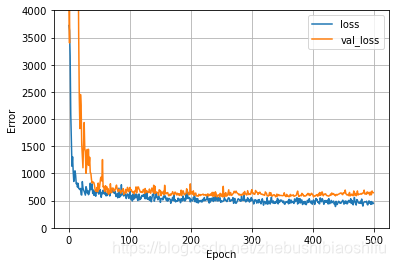
机器学习中,过拟合是影响训练精度的重要因素。因此,我们最好在训练模型的过程中绘制训练数据、验证数据的误差变化图象,从而更好获取模型的训练情况。
# Draw error image.
def LossPlot(History):
    plt.figure(2)
    plt.plot(History.history['loss'],label='loss')
    plt.plot(History.history['val_loss'],label='val_loss')
    plt.ylim([0,4000])
    plt.xlabel('Epoch')
    plt.ylabel('Error')
    plt.legend()
    plt.grid(True)

# Draw error image.
LossPlot(DNNHistory)
其中,'loss'与'val_loss'分别是模型训练过程中,训练集、验证集对应的误差;如果训练集误差明显小于验证集误差,就说明模型出现了过拟合。
前面提到了,我们将多个符合要求的Epoch保存在了指定的路径下,那么最终我们可以从中选取最好的那个Epoch,作为模型的最终参数,从而对测试集数据加以预测。那么在这里,我们需要将这一全局最优Epoch选取出,并带入到最终的模型里。
# Optimize the model based on optimal epoch.
def BestEpochIntoModel(Path,Model):
    EpochFile=glob.glob(Path+'/*')
    BestEpoch=max(EpochFile,key=os.path.getmtime)
    Model.load_weights(BestEpoch)
    Model.compile(loss=LossMethod,
                  optimizer=BestEpochOptMethod)
    return Model

# Optimize the model based on optimal epoch.
DNNModel=BestEpochIntoModel(CheckPointPath,DNNModel)
总的来说,这里就是运用了os.path.getmtime模块,将我们存储Epoch的文件夹中最新的那个Epoch挑出来——这一Epoch就是使得验证集数据误差最小的全局最优Epoch;并通过load_weights将这一Epoch对应的模型参数引入模型。
前期一篇文章Python TensorFlow深度学习回归代码:DNNRegressor中有相关的代码讲解内容,因此这里就不再赘述啦。
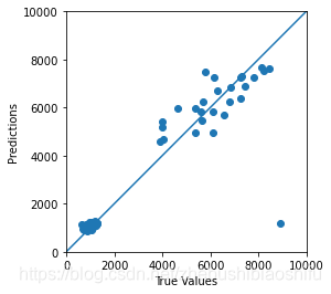
# Draw Test image.
def TestPlot(TestY,TestPrediction):
plt.figure(3)
ax=plt.axes(aspect='equal')
plt.scatter(TestY,TestPrediction)
plt.xlabel('True Values')
plt.ylabel('Predictions')
Lims=[0,10000]
plt.xlim(Lims)
plt.ylim(Lims)
plt.plot(Lims,Lims)
plt.grid(False)
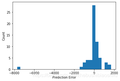
# Verify the accuracy and draw error hist image.
def AccuracyVerification(TestY,TestPrediction):
DNNError=TestPrediction-TestY
plt.figure(4)
plt.hist(DNNError,bins=30)
plt.xlabel('Prediction Error')
plt.ylabel('Count')
plt.grid(False)
Pearsonr=stats.pearsonr(TestY,TestPrediction)
R2=metrics.r2_score(TestY,TestPrediction)
RMSE=metrics.mean_squared_error(TestY,TestPrediction)**0.5
print('Pearson correlation coefficient is {0}, and RMSE is {1}.'.format(Pearsonr[0],RMSE))
return (Pearsonr[0],R2,RMSE)
# Save key parameters.
def WriteAccuracy(*WriteVar):
ExcelData=openpyxl.load_workbook(WriteVar[0])
SheetName=ExcelData.get_sheet_names()
WriteSheet=ExcelData.get_sheet_by_name(SheetName[0])
WriteSheet=ExcelData.active
MaxRowNum=WriteSheet.max_row
for i in range(len(WriteVar)-1):
exec("WriteSheet.cell(MaxRowNum+1,i+1).value=WriteVar[i+1]")
ExcelData.save(WriteVar[0])
# Predict test set data.
TestPrediction=DNNModel.predict(TestX).flatten()
# Draw Test image.
TestPlot(TestY,TestPrediction)
# Verify the accuracy and draw error hist image.
AccuracyResult=AccuracyVerification(TestY,TestPrediction)
PearsonR,R2,RMSE=AccuracyResult[0],AccuracyResult[1],AccuracyResult[2]
# Save model and key parameters.
DNNModel.save(ModelPath)
WriteAccuracy(ParameterPath,PearsonR,R2,RMSE,TrainFrac,RandomSeed,CheckPointMethod,
','.join('%s' %i for i in HiddenLayer),RegularizationFactor,
ActivationMethod,','.join('%s' %i for i in DropoutValue),OutputLayerActMethod,
LossMethod,LearnRate,LearnDecay,FitEpoch,BatchSize,ValFrac,BestEpochOptMethod)
得到拟合图像如下:
得到误差分布直方图如下:
至此,代码的分解介绍就结束啦~
# -*- coding: utf-8 -*-
"""
Created on Tue Feb 24 12:42:17 2021

@author: fkxxgis
"""

import os
import glob
import openpyxl
import numpy as np
import pandas as pd
import seaborn as sns
import tensorflow as tf
import scipy.stats as stats
import matplotlib.pyplot as plt
from sklearn import metrics
from tensorflow import keras
from tensorflow.keras import layers
from tensorflow.keras import regularizers
from tensorflow.keras.callbacks import ModelCheckpoint
from tensorflow.keras.layers.experimental import preprocessing

np.set_printoptions(precision=4,suppress=True)

# Draw the joint distribution image.
def JointDistribution(Factors):
    plt.figure(1)
    sns.pairplot(TrainData[Factors],kind='reg',diag_kind='kde')
    sns.set(font_scale=2.0)
    DataDistribution=TrainData.describe().transpose()

# Delete the model result from the last run.
def DeleteOldModel(ModelPath):
    AllFileName=os.listdir(ModelPath)
    for i in AllFileName:
        NewPath=os.path.join(ModelPath,i)
        if os.path.isdir(NewPath):
            DeleteOldModel(NewPath)
        else:
            os.remove(NewPath)

# Find and save optimal epoch.
def CheckPoint(Name):
    Checkpoint=ModelCheckpoint(Name,
                               monitor=CheckPointMethod,
                               verbose=1,
                               save_best_only=True,
                               mode='auto')
    CallBackList=[Checkpoint]
    return CallBackList

# Build DNN model.
def BuildModel(Norm):
    Model=keras.Sequential([Norm, # 数据标准化层

                            layers.Dense(HiddenLayer[0], # 指定隐藏层1的神经元个数
                                         kernel_regularizer=regularizers.l2(RegularizationFactor), # 运用L2正则化
                                         # activation=ActivationMethod
                                         ),
                            layers.LeakyReLU(), # 引入LeakyReLU这一改良的ReLU激活函数,从而加快模型收敛,减少过拟合
                            layers.BatchNormalization(), # 引入Batch Normalizing,加快网络收敛与增强网络稳固性
                            layers.Dropout(DropoutValue[0]), # 指定隐藏层1的Dropout值

                            layers.Dense(HiddenLayer[1],
                                         kernel_regularizer=regularizers.l2(RegularizationFactor),
                                         # activation=ActivationMethod
                                         ),
                            layers.LeakyReLU(),
                            layers.BatchNormalization(),
                            layers.Dropout(DropoutValue[1]),

                            layers.Dense(HiddenLayer[2],
                                         kernel_regularizer=regularizers.l2(RegularizationFactor),
                                         # activation=ActivationMethod
                                         ),
                            layers.LeakyReLU(),
                            layers.BatchNormalization(),
                            layers.Dropout(DropoutValue[2]),

                            layers.Dense(HiddenLayer[3],
                                         kernel_regularizer=regularizers.l2(RegularizationFactor),
                                         # activation=ActivationMethod
                                         ),
                            layers.LeakyReLU(),
                            layers.BatchNormalization(),
                            layers.Dropout(DropoutValue[3]),

                            layers.Dense(HiddenLayer[4],
                                         kernel_regularizer=regularizers.l2(RegularizationFactor),
                                         # activation=ActivationMethod
                                         ),
                            layers.LeakyReLU(),
                            layers.BatchNormalization(),
                            layers.Dropout(DropoutValue[4]),

                            layers.Dense(HiddenLayer[5],
                                         kernel_regularizer=regularizers.l2(RegularizationFactor),
                                         # activation=ActivationMethod
                                         ),
                            layers.LeakyReLU(),
                            layers.BatchNormalization(),
                            layers.Dropout(DropoutValue[5]),

                            layers.Dense(HiddenLayer[6],
                                         kernel_regularizer=regularizers.l2(RegularizationFactor),
                                         # activation=ActivationMethod
                                         ),
                            layers.LeakyReLU(),
                            # If batch normalization is set in the last hidden layer, the error image
                            # will show a trend of first stable and then decline; otherwise, it will
                            # decline and then stable.
                            # layers.BatchNormalization(),
                            layers.Dropout(DropoutValue[6]),

                            layers.Dense(units=1,
                                         activation=OutputLayerActMethod)]) # 最后一层就是输出层
    Model.compile(loss=LossMethod, # 指定每个批次训练误差的减小方法
                  optimizer=tf.keras.optimizers.Adam(learning_rate=LearnRate,decay=LearnDecay))
                  # 运用学习率下降的优化方法
    return Model

# Draw error image.
def LossPlot(History):
    plt.figure(2)
    plt.plot(History.history['loss'],label='loss')
    plt.plot(History.history['val_loss'],label='val_loss')
    plt.ylim([0,4000])
    plt.xlabel('Epoch')
    plt.ylabel('Error')
    plt.legend()
    plt.grid(True)

# Optimize the model based on optimal epoch.
def BestEpochIntoModel(Path,Model):
    EpochFile=glob.glob(Path+'/*')
    BestEpoch=max(EpochFile,key=os.path.getmtime)
    Model.load_weights(BestEpoch)
    Model.compile(loss=LossMethod,
                  optimizer=BestEpochOptMethod)
    return Model

# Draw Test image.
def TestPlot(TestY,TestPrediction):
    plt.figure(3)
    ax=plt.axes(aspect='equal')
    plt.scatter(TestY,TestPrediction)
    plt.xlabel('True Values')
    plt.ylabel('Predictions')
    Lims=[0,10000]
    plt.xlim(Lims)
    plt.ylim(Lims)
    plt.plot(Lims,Lims)
    plt.grid(False)

# Verify the accuracy and draw error hist image.
def AccuracyVerification(TestY,TestPrediction):
    DNNError=TestPrediction-TestY
    plt.figure(4)
    plt.hist(DNNError,bins=30)
    plt.xlabel('Prediction Error')
    plt.ylabel('Count')
    plt.grid(False)
    Pearsonr=stats.pearsonr(TestY,TestPrediction)
    R2=metrics.r2_score(TestY,TestPrediction)
    RMSE=metrics.mean_squared_error(TestY,TestPrediction)**0.5
    print('Pearson correlation coefficient is {0}, and RMSE is {1}.'.format(Pearsonr[0],RMSE))
    return (Pearsonr[0],R2,RMSE)

# Save key parameters.
def WriteAccuracy(*WriteVar):
    ExcelData=openpyxl.load_workbook(WriteVar[0])
    SheetName=ExcelData.get_sheet_names()
    WriteSheet=ExcelData.get_sheet_by_name(SheetName[0])
    WriteSheet=ExcelData.active
    MaxRowNum=WriteSheet.max_row
    for i in range(len(WriteVar)-1):
        exec("WriteSheet.cell(MaxRowNum+1,i+1).value=WriteVar[i+1]")
    ExcelData.save(WriteVar[0])

# Input parameters.
DataPath="G:/CropYield/03_DL/00_Data/AllDataAll.csv"
ModelPath="G:/CropYield/03_DL/02_DNNModle"
CheckPointPath="G:/CropYield/03_DL/02_DNNModle/Weights"
CheckPointName=CheckPointPath+"/Weights_{epoch:03d}_{val_loss:.4f}.hdf5"
ParameterPath="G:/CropYield/03_DL/03_OtherResult/ParameterResult.xlsx"
TrainFrac=0.8
RandomSeed=np.random.randint(low=21,high=22)
CheckPointMethod='val_loss'
HiddenLayer=[64,128,256,512,512,1024,1024]
RegularizationFactor=0.0001
ActivationMethod='relu'
DropoutValue=[0.5,0.5,0.5,0.3,0.3,0.3,0.2]
OutputLayerActMethod='linear'
LossMethod='mean_absolute_error'
LearnRate=0.005
LearnDecay=0.0005
FitEpoch=500
BatchSize=9999
ValFrac=0.2
BestEpochOptMethod='adam'

# Fetch and divide data.
MyData=pd.read_csv(DataPath,names=['EVI0610','EVI0626','EVI0712','EVI0728','EVI0813','EVI0829',
                                   'EVI0914','EVI0930','EVI1016','Lrad06','Lrad07','Lrad08',
                                   'Lrad09','Lrad10','Prec06','Prec07','Prec08','Prec09',
                                   'Prec10','Pres06','Pres07','Pres08','Pres09','Pres10',
                                   'SIF161','SIF177','SIF193','SIF209','SIF225','SIF241',
                                   'SIF257','SIF273','SIF289','Shum06','Shum07','Shum08',
                                   'Shum09','Shum10','SoilType','Srad06','Srad07','Srad08',
                                   'Srad09','Srad10','Temp06','Temp07','Temp08','Temp09',
                                   'Temp10','Wind06','Wind07','Wind08','Wind09','Wind10',
                                   'Yield'],header=0)
TrainData=MyData.sample(frac=TrainFrac,random_state=RandomSeed)
TestData=MyData.drop(TrainData.index)

# Draw the joint distribution image.
# JointFactor=['Lrad07','Prec06','SIF161','Shum06','Srad07','Srad08','Srad10','Temp06','Yield']
# JointDistribution(JointFactor)

# Separate independent and dependent variables.
TrainX=TrainData.copy(deep=True)
TestX=TestData.copy(deep=True)
TrainY=TrainX.pop('Yield')
TestY=TestX.pop('Yield')

# Standardization data.
Normalizer=preprocessing.Normalization()
Normalizer.adapt(np.array(TrainX))

# Delete the model result from the last run.
DeleteOldModel(ModelPath)

# Find and save optimal epochs.
CallBack=CheckPoint(CheckPointName)

# Build DNN regression model.
DNNModel=BuildModel(Normalizer)
DNNModel.summary()
DNNHistory=DNNModel.fit(TrainX,
                        TrainY,
                        epochs=FitEpoch,
                        # batch_size=BatchSize,
                        verbose=1,
                        callbacks=CallBack,
                        validation_split=ValFrac)

# Draw error image.
LossPlot(DNNHistory)

# Optimize the model based on optimal epoch.
DNNModel=BestEpochIntoModel(CheckPointPath,DNNModel)

# Predict test set data.
TestPrediction=DNNModel.predict(TestX).flatten()

# Draw Test image.
TestPlot(TestY,TestPrediction)

# Verify the accuracy and draw error hist image.
AccuracyResult=AccuracyVerification(TestY,TestPrediction)
PearsonR,R2,RMSE=AccuracyResult[0],AccuracyResult[1],AccuracyResult[2]

# Save model and key parameters.
DNNModel.save(ModelPath)
WriteAccuracy(ParameterPath,PearsonR,R2,RMSE,TrainFrac,RandomSeed,CheckPointMethod,
              ','.join('%s' %i for i in HiddenLayer),RegularizationFactor,
              ActivationMethod,','.join('%s' %i for i in DropoutValue),OutputLayerActMethod,
              LossMethod,LearnRate,LearnDecay,FitEpoch,BatchSize,ValFrac,BestEpochOptMethod)
至此,大功告成。
我想在Ruby中创建一个用于开发目的的极其简单的Web服务器(不,不想使用现成的解决方案)。代码如下:#!/usr/bin/rubyrequire'socket'server=TCPServer.new('127.0.0.1',8080)whileconnection=server.acceptheaders=[]length=0whileline=connection.getsheaders想法是从命令行运行这个脚本,提供另一个脚本,它将在其标准输入上获取请求,并在其标准输出上返回完整的响应。到目前为止一切顺利,但事实证明这真的很脆弱,因为它在第二个请求上中断并出现错误:/usr/b
网络编程套接字网络编程基础知识理解源`IP`地址和目的`IP`地址理解源MAC地址和目的MAC地址认识端口号理解端口号和进程ID理解源端口号和目的端口号认识`TCP`协议认识`UDP`协议网络字节序socket编程接口`sockaddr``UDP`网络程序服务器端代码逻辑:需要用到的接口服务器端代码`udp`客户端代码逻辑`udp`客户端代码`TCP`网络程序服务器代码逻辑多个版本服务器单进程版本多进程版本多线程版本线程池版本服务器端代码客户端代码逻辑客户端代码TCP协议通讯流程TCP协议的客户端/服务器程序流程三次握手(建立连接)数据传输四次挥手(断开连接)TCP和UDP对比网络编程基础知识
深度学习部署:Windows安装pycocotools报错解决方法1.pycocotools库的简介2.pycocotools安装的坑3.解决办法更多Ai资讯:公主号AiCharm本系列是作者在跑一些深度学习实例时,遇到的各种各样的问题及解决办法,希望能够帮助到大家。ERROR:Commanderroredoutwithexitstatus1:'D:\Anaconda3\python.exe'-u-c'importsys,setuptools,tokenize;sys.argv[0]='"'"'C:\\Users\\46653\\AppData\\Local\\Temp\\pip-instal
是否可以在不实际下载文件的情况下检查文件是否存在?我有这么大的(~40mb)文件,例如:http://mirrors.sohu.com/mysql/MySQL-6.0/MySQL-6.0.11-0.glibc23.src.rpm这与ruby不严格相关,但如果发件人可以设置内容长度就好了。RestClient.get"http://mirrors.sohu.com/mysql/MySQL-6.0/MySQL-6.0.11-0.glibc23.src.rpm",headers:{"Content-Length"=>100} 最佳答案
我在这方面尝试了很多URL,在我遇到这个特定的之前,它们似乎都很好:require'rubygems'require'nokogiri'require'open-uri'doc=Nokogiri::HTML(open("http://www.moxyst.com/fashion/men-clothing/underwear.html"))putsdoc这是结果:/Users/macbookair/.rvm/rubies/ruby-2.0.0-p481/lib/ruby/2.0.0/open-uri.rb:353:in`open_http':404NotFound(OpenURI::HT
深度学习12.CNN经典网络VGG16一、简介1.VGG来源2.VGG分类3.不同模型的参数数量4.3x3卷积核的好处5.关于学习率调度6.批归一化二、VGG16层分析1.层划分2.参数展开过程图解3.参数传递示例4.VGG16各层参数数量三、代码分析1.VGG16模型定义2.训练3.测试一、简介1.VGG来源VGG(VisualGeometryGroup)是一个视觉几何组在2014年提出的深度卷积神经网络架构。VGG在2014年ImageNet图像分类竞赛亚军,定位竞赛冠军;VGG网络采用连续的小卷积核(3x3)和池化层构建深度神经网络,网络深度可以达到16层或19层,其中VGG16和VGG
(本文是网络的宏观的概念铺垫)目录计算机网络背景网络发展认识"协议"网络协议初识协议分层OSI七层模型TCP/IP五层(或四层)模型报头以太网碰撞路由器IP地址和MAC地址IP地址与MAC地址总结IP地址MAC地址计算机网络背景网络发展 是最开始先有的计算机,计算机后来因为多项技术的水平升高,逐渐的计算机变的小型化、高效化。后来因为计算机其本身的计算能力比较的快速:独立模式:计算机之间相互独立。 如:有三个人,每个人做的不同的事物,但是是需要协作的完成。 而这三个人所做的事是需要进行协作的,然而刚开始因为每一台计算机之间都是互相独立的。所以前面的人处理完了就需要将数据
安全产品安全网关类防火墙Firewall防火墙防火墙主要用于边界安全防护的权限控制和安全域的划分。防火墙•信息安全的防护系统,依照特定的规则,允许或是限制传输的数据通过。防火墙是一个由软件和硬件设备组合而成,在内外网之间、专网与公网之间的界面上构成的保护屏障。下一代防火墙•下一代防火墙,NextGenerationFirewall,简称NGFirewall,是一款可以全面应对应用层威胁的高性能防火墙,提供网络层应用层一体化安全防护。生产厂家•联想网御、CheckPoint、深信服、网康、天融信、华为、H3C等防火墙部署部署于内、外网编辑额,用于权限访问控制和安全域划分。UTM统一威胁管理(Un
Linux操作系统——网络配置与SSH远程安装完VMware与系统后,需要进行网络配置。第一个目标为进行SSH连接,可以从本机到VMware进行文件传送,首先需要进行网络配置。1.下载远程软件首先需要先下载安装一款远程软件:FinalShell或者xhell7FinalShellxhell7FinalShell下载:Windows下载http://www.hostbuf.com/downloads/finalshell_install.exemacOS下载http://www.hostbuf.com/downloads/finalshell_install.pkg2.配置CentOS网络安装好
在神经网络方面,我完全是个初学者。我整天都在与ruby-fann和ai4r搏斗,不幸的是我没有任何东西可以展示,所以我想我会来到StackOverflow并询问这里的知识渊博的人。我有一组样本——每天都有一个数据点,但它们不符合我能够找出的任何明确模式(我尝试了几次回归)。不过,我认为看看是否有任何方法可以仅从日期预测future的数据会很好,而且我认为神经网络将是生成希望表达这种关系的函数的好方法.日期是DateTime对象,数据点是十进制数,例如7.68。我一直在将DateTime对象转换为float,然后除以10,000,000,000得到一个介于0和1之间的数字,我一直在将