一：boston数据集

    Boston数据集各个特征的含义如下：

特征值	特征值含义
CRIM	城镇人均犯罪率
ZN	住宅用地所占比例
INDUS	城镇中非住宅用地所占比例
CHAS	虚拟变量,用于回归分析
NOX	环保指数
RM	每栋住宅的房间数
AGE	1940 年以前建成的自住单位的比例
DIS	距离 5 个波士顿的就业中心的加权距离
RAD	距离高速公路的便利指数
TAX	每一万美元的不动产税率
PTRATIO	城镇中的教师学生比例
B	城镇中的黑人比例
LSTAT	地区中有多少房东属于低收入人群
MEDV	自住房屋房价中位数（也就是均价）

   

波士顿房价数据集包括506个样本，每个样本包括12个特征变量和该地区的平均房价，房价显然和多个特征变量相关，先选择亿元线性回归与多个特征建立线性方程，观察模型预测的好坏，再选择多元线性回归进行房价预测。

建立线性模型

二：boston数据处理及模型建立

2.1加载boston数据集

import pandas as pd

import numpy as np

import matplotlib

matplotlib.rcParams['font.sans-serif'] = ['SimHei']

matplotlib.rcParams['font.family'] = 'sans-serif'

matplotlib.rcParams['axes.unicode_minus'] = False

import matplotlib.pyplot as plt

from sklearn import datasets

# 获取数据

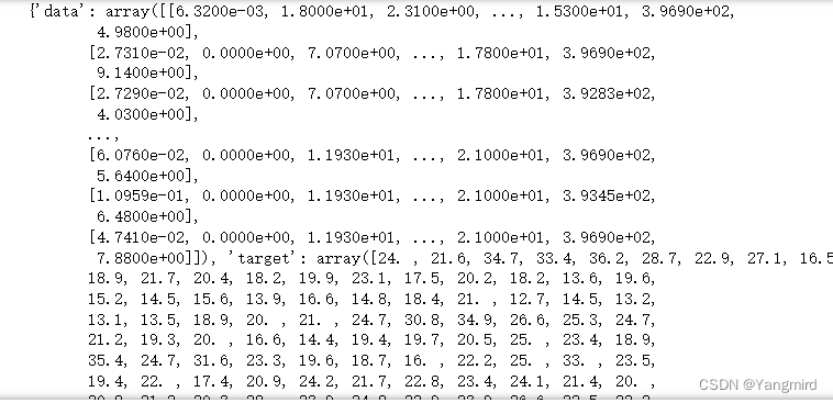
boston = datasets.load_boston()

print(boston)

boston_df = pd.DataFrame(boston.data, columns=boston.feature_names)

boston_df['MEDV'] = boston.target  # 房价-----y

    查看数据:

# 查看数据是否存在空值，从结果来看数据不存在空值。

boston_df.isnull().sum()

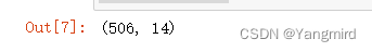
可以看出，boston数据集中有14个特征，并且没有缺失值，所以不用做缺失值处理，其中’MEDV’作为目标值。

# 查看数据大小

boston_df.shape

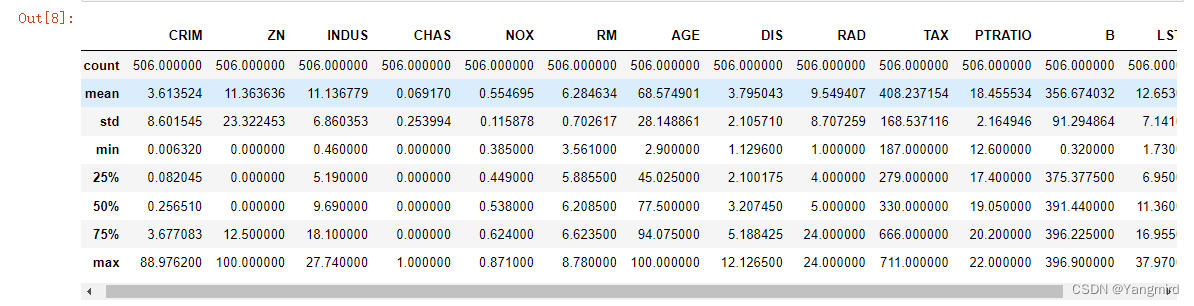
# 查看数据的描述信息，在描述信息里可以看到每个特征的均值，最大值，最小值等信息。

boston_df.describe()

# 看看各个特征中是否有相关性，判断一下用哪种模型比较合适

import seaborn as sns

plt.figure(figsize=(12,8))

sns.heatmap(boston_df.corr(), annot=True, fmt='.2f',cmap='PuBu')

从上图可以看出数据不存在相关性较小的属性，也不用担心共线性，所以可以用线性回归模型去预测。

2.2 画出各个特征与MEDV房价的散点图

   # 各个特征和MEDV房价的散点图

boston_df_xTitle=['CRIM','ZN','INDUS','CHAS','NOX','RM','AGE','DIS','RAD','TAX','PTRATIO','B','LSTAT']

for i in range(0,len(boston_df_xTitle)):

      plt.figure(facecolor='white')

          plt.scatter(boston_df[str(boston_df_xTitle[i])], boston_df['MEDV'], s=30, edgecolor='white')

    plt.title(str(boston_df_xTitle[i])+'--------MEDV')

    plt.xlabel(str(boston_df_xTitle[i]))

    plt.ylabel('MEDV房价')

    plt.show()

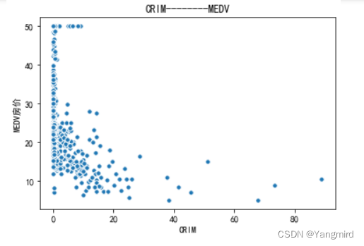
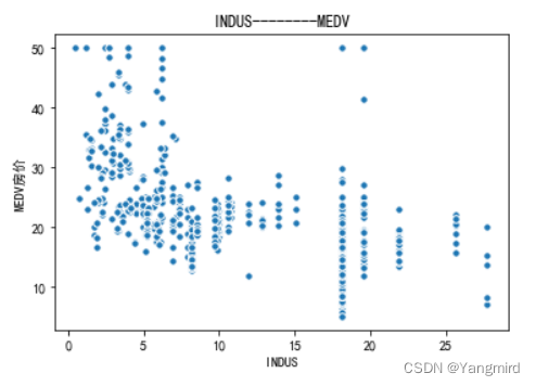
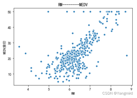
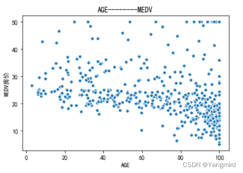
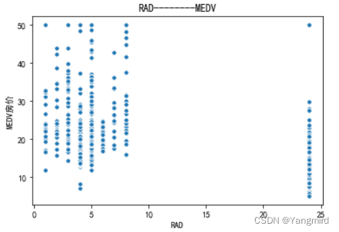
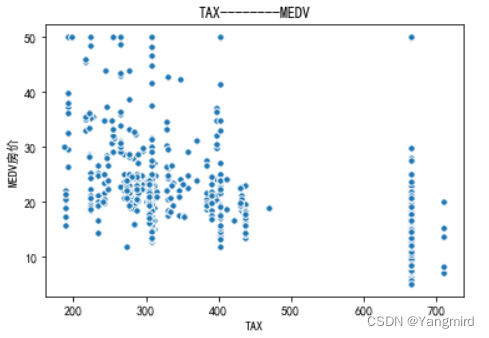
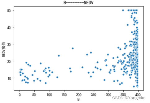
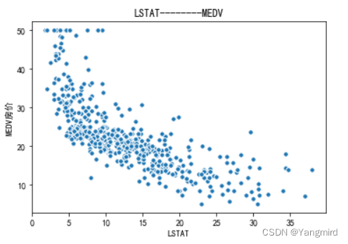
从上图可以看出’RM’,’LSTAT’,’CRIM’这三个特征值与房价存在一定的相关性，所以选择该三个特征作为特征值，移除其余不相关的特征值。

# 定义目标值和特征值

# 分析房屋的’RM’， ‘LSTAT’，'CRIM’ 特征与MEDV的相关性性，所以，将其余不相关特征移除

new_boston_df = boston_df[['LSTAT', 'CRIM', 'RM', 'MEDV']]

# print('describe:      ')

# new_boston_df.describe()

#  目标值

y = np.array(new_boston_df['MEDV'])

# drop函数默认删除行，列需要加axis=1

new_boston_df = new_boston_df.drop(['MEDV'], axis=1)

# 特征值

X = np.array(new_boston_df)

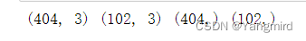
2.3划分训练集和测试集

由于数据没有null值，并且，都是连续型数据，所以暂时不用对数据进行过多的处理，不够既然要建立模型，首先就要进行对boston数据集分为训练集和测试集，取出了大概百分之30的数据作为测试集，剩下的百分之70为训练集

# 划分训练集和测试集

from sklearn.model_selection import train_test_split

# 70%用于训练，30%用于测试

X_train, X_test, y_train, y_test = train_test_split(X, y, test_size=0.2, random_state=10)

print(X_train.shape, X_test.shape, y_train.shape, y_test.shape)

2.4建立线性回归模型

 # 线性回归-------------------------------------------------

from sklearn.linear_model import LinearRegression

from sklearn.preprocessing import StandardScaler

lr = LinearRegression()

# ss=StandardScaler()

# 使用训练数据进行参数估计

lr.fit(X_train, y_train)

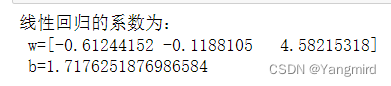
# 输出线性回归的系数

print('线性回归的系数为：\n w=%s\n b=%s ' % (lr.coef_, lr.intercept_))

lr_reg_pre=lr.predict(X_test)

# -----------------------------------------------------------

2.5计算MAE和MSE

# 进行预测

# 使用测试数据进行回归预测

y_test_pred = lr.predict(X_test)

print('y_test_pred:\n', y_test_pred)

# 训练数据的预测值

y_train_pred = lr.predict(X_train)

print('y_train_pred : \n ', y_train_pred)

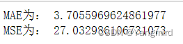
# 计算平均绝对误差MAE

train_MAE=mean_absolute_error(y_train,y_train_pred)

print('MAE为：',train_MAE)

#  计算均方误差MSE

train_MSE=mean_squared_error(y_train,y_train_pred) # 训练值与训练预测值之间的对比

print('MSE为：',train_MSE)

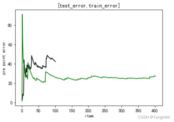
# 绘制MAE和MSE图

2.6画出学习曲线

    from sklearn.model_selection import  learning_curve,ShuffleSplit

def plot_learning_curve(plt,estimator,title,X,y,

ylim=None,cv=None,n_jobs=1,train_sizes=np.linspace(.1,1.0,5)):

      plt.title(title)

      if ylim is not None:

         plt.ylim(ylim)

      plt.xlabel("Training examples")

      plt.ylabel("Score")

train_sizes,train_scores,test_scores=learning_curve(estimator,X,y,cv=cv,n_jobs=n_jobs,train_sizes=train_sizes)

     train_scores_mean=np.mean(train_scores,axis=1)

     train_scores_std=np.std(train_scores,axis=1)

     test_scores_mean=np.mean(test_scores,axis=1)

     test_scores_std=np.std(test_scores,axis=1)

     plt.grid()

     plt.fill_between(train_sizes,train_scores_mean-train_scores_std,train_scores_mean+train_scores_std,alpha=0.1,color="r")

     plt.fill_between(train_sizes,test_scores_mean-test_scores_std,test_scores_mean+test_scores_std,alpha=0.1,color="g")

     plt.plot(train_sizes,train_scores_mean,'o--',color="r",label="Training scores")

     plt.plot(train_sizes,test_scores_mean,'o-',color="g",label="Cross-validation score")

     plt.legend(loc="best")

     return plt

cv=ShuffleSplit(n_splits=10,test_size=0.2,random_state=0)

plt.figure(figsize=(10,6))

plot_learning_curve(plt,lr,"Learn Curve for LinearRegression",new_boston_df,y,ylim=None,cv=cv)

plt.show()

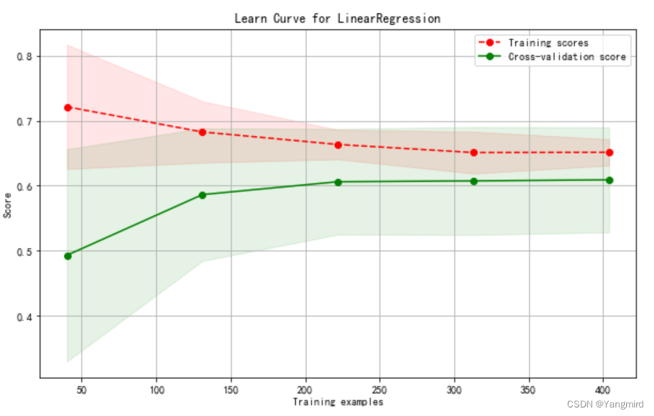
    可以看出，模型有些欠拟合，需要优化，考虑使用二项式、三项式进行优化。

三：模型优化及结果分析

3.1模型优化

    # 定义划分数据集函数

def split_data():

    X=boston.data

    y=boston.target

    print(boston.feature_names)

    X_train, X_test, y_train, y_test = train_test_split(X, y, test_size=0.2, random_state=2)

    return (X, y, X_train, X_test, y_train, y_test)

# 定义MAE函数

def mae_value(y_train,y_train_pred):

    n=len(y_train)

    mae=mean_absolute_error(y_train,y_train_pred)

    return  mae

# 定义MSE函数

def mse_value(y_train,y_train_pred):

    n=len(y_train)

    mse=mean_squared_error(y_train,y_train_pred)

    return  mse

# 定义多项式模型函数

from sklearn.preprocessing import PolynomialFeatures

from sklearn.pipeline import Pipeline

def polynomial_regression(degree=1):

    polynomial_features=PolynomialFeatures(degree=degree,include_bias=False)

    # 模型开启数据归一化

    linear_regression_model=LinearRegression(normalize=True)

    model=Pipeline([("polynomial_features", polynomial_features),

                    ("linear_regression", linear_regression_model)])

    return  model

# 训练模型

def train_model(X_train, X_test, y_train, y_test,degrees):

    res=[]

    for degree in degrees:

        model=polynomial_regression(degree)

        model.fit(X_train,y_train)

        train_score=model.score(X_train,y_train)*100

        test_score = model.score(X_test, y_test)*100

        res.append({'model':model,'degree':degree,'train_score':train_score,'test_score':test_score})

        y_test_predict=model.predict(X_test)

        mae=mae_value(y_test,y_test_predict)

        mse=mse_value(y_test,y_test_predict)

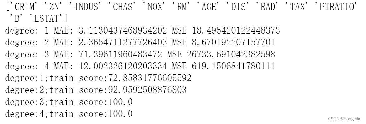
        print("degree:",degree, "MAE:",mae,"MSE",mse)

    for r in res:

        print("degree:{};train_score:{}".format(r["degree"],r["train_score"],r["test_score"]))

    return res

# 定义画出学习曲线的函数

from sklearn.model_selection import learning_curve

def plot_learning_curve(plt,estimator,title,X,y,ylim=None,cv=None,n_jobs=1,train_sizes=np.linspace(.1,1.0,5)):

   plt.title(title)

   if ylim is not None:

     plt.ylim(ylim)

   plt.xlabel("Training examples")

   plt.ylabel("Score")

   train_sizes,train_scores,test_scores=learning_curve(estimator,X,y,cv=cv,n_jobs=n_jobs,train_sizes=train_sizes)

    train_scores_mean=np.mean(train_scores,axis=1)

    train_scores_std=np.std(train_scores,axis=1)

    test_scores_mean=np.mean(test_scores,axis=1)

    test_scores_std=np.std(test_scores,axis=1)

    plt.grid()

  plt.fill_between(train_sizes,train_scores_mean-train_scores_std,train_scores_mean+train_scores_std,alpha=0.1,color="r")

   plt.fill_between(train_sizes,test_scores_mean-test_scores_std,test_scores_mean+test_scores_std,alpha=0.1,color="g")

   plt.plot(train_sizes,train_scores_mean,'o--',color="r",label="Training scores")

   plt.plot(train_sizes,test_scores_mean,'o-',color="g",label="Cross-validation score")

   plt.legend(loc="best")

   return plt

# 定义1、2、3次多项式

degrees=[1,2,3,4]

# 划分数据集

X, y, X_train, X_test, y_train, y_test = split_data()

#训练模型，并打印train score

res = train_model(X_train, X_test, y_train, y_test, degrees)

# 画出学习曲线

from sklearn.model_selection import ShuffleSplit

cv=ShuffleSplit(n_splits=10, test_size=0.2, random_state=0)

plt.figure(figsize=(10,6))

for index,data in enumerate(res):

 plot_learning_curve(plt,data["model"],"degree%d"%data["degree"],X,y,cv=cv)

   plt.show()

3.2结果分析

    模型优化结果如下：

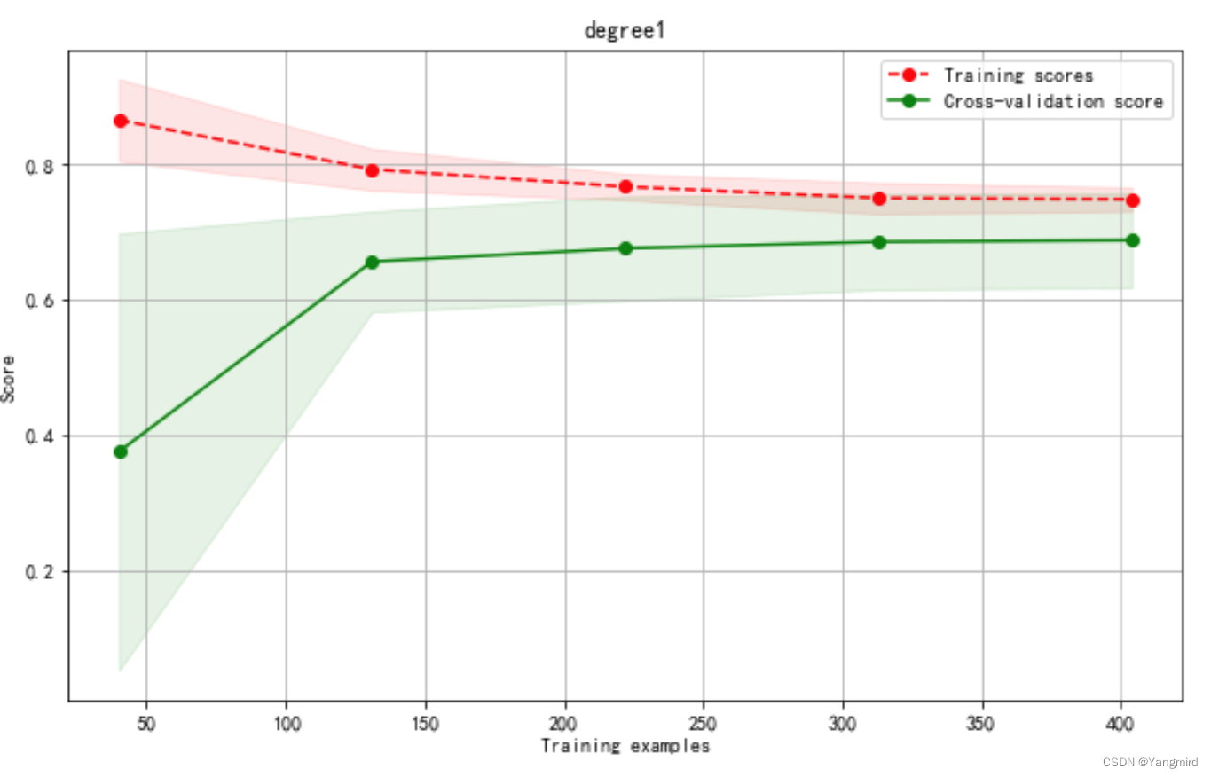
    Degree=1时学习曲线如下:

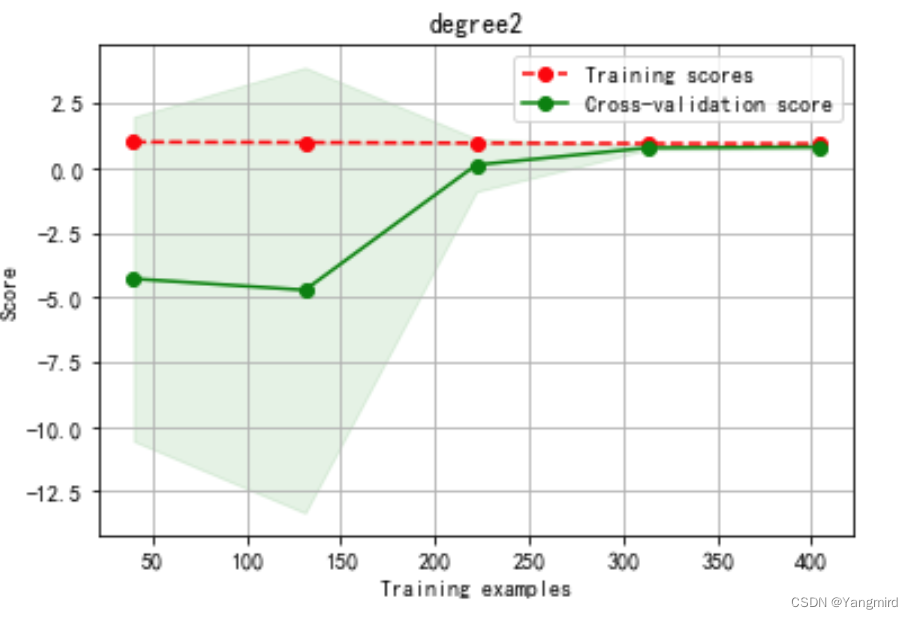
Degree=2时学习曲线如下:

Degree=3时学习曲线如下:

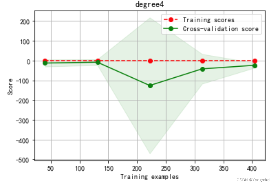
Degree=4时学习曲线如下:

    根据上述模型优化结果分析可知，二次多项式效果较好，训练准确度达到了92.9%,MAE=2.36,MSE=8.67,比一次多项式的训练准确度72.8%要更准确。